Many papers present formulae to price Asian options in the Black-Scholes world only for the fixed strike Asian case, that is
a contract that pays \( \max(A-K,0)\) at maturity \(T\) where \(A = \sum_{i=0}^{n-1} w_i S(t_i) \) is the Asian average.
More generally, this can be seen as the payoff of a Basket option where the underlyings are just the same asset but at different times.
And any Basket option formula can actually be used to price fixed-strike Asian options by letting the correlation correspond to the correlation between the asset at the averaging times
and the variances correspond to the variance at each averaging time. The basket approach allows then naturally for a term-structure of rates, dividends and volatilities.
We have:
$$
V_{\textsf{floating}}(\eta,S_0,k,\bar{\sigma}_i^2 t_i, C(0,t_i), B(0,T)) =\\
\quad k V_{\textsf{fixed}}\left(-\eta,S_0, \frac{S_0}{k},\bar{\sigma}^2(T) T-\bar{\sigma}_i^2 t_i,\frac{C(0,t_i)}{C(0,T)},B(0,T)C(0,T) \right)
$$
where \(\eta = \pm 1\) for a call (respectively a put), \(\bar{\sigma}_i\) are the Vanilla options implied volatilities at the averaging times \(t_i\), \(C(0,t_i)\) are the capitalization factors, and \(B(0,T)\) is the discount factor.
Proof:
We assume that \(S\) follows \(dS = \mu_t S dt + \sigma_t S dW_t\). The discount factor \(B\) is defined as \(B(0,T)=e^{-\int_{0}^T r_s ds}\). Let \(C(0,t) = e^{\int_{0}^t \mu_s ds}\). The process associated to the forward to time \(t\) is \(F_t=S_0 C(0,t)M_t\) with \(M_t = e^{\int_0^t \sigma_s dW_s - \frac{1}{2}\int_0^t \sigma_s^2 ds}\) being a martingale.
We have:
$$
V_{\textsf{floating}}(\eta,S_0,k,\bar{\sigma}_i^2 t_i, C(0,t_i), B(0,T))\\
= B(0,T)\mathbb{E}\left[\max\left(\eta F_T-\eta k\sum_{i=0}^{n-1}w_i F_{t_i},0\right)\right]\\
= k B(0,T)\mathbb{E}\left[\max\left(\eta\frac{1}{k}F_T-\eta\sum_{i=0}^{n-1}w_i F_{t_i},0\right)\right]\\
=k B(0,T)C(0,T)\mathbb{E}\left[ M_T \max\left(\eta\frac{S_0}{k}-\eta\sum_{i=0}^{n-1}w_i S_0 \frac{C(0,t_i)M_{t_i}}{C(0,T) M_T },0\right)\right]
$$
We now proceed to a change of measure defined by \(M_T\). Under the new measure \(\mathbb{Q}^T\), \(\bar{W}_t = W_t - \int_0^t \sigma_s ds\) is a Brownian motion. \(\frac{M_t}{M_T}\) under \(\mathbb{Q}\) has the same law as \(\frac{M_t}{M_T} e^{-\int_t^T \sigma_s^2 ds}\) under \(\mathbb{Q}^T\) or equivalently as
\(\bar{M}_t = e^{\int_t^T \sigma_s d\bar{W}_s - \frac{1}{2}\int_t^T \sigma_s^2 ds}\) under \(\mathbb{Q}^T\).
Defining \(\mathbb{E}^T\) to be the expectation under \(\mathbb{Q}^T\), we thus have
$$
V_{\textsf{floating}}(\eta,S,k,\bar{\sigma}_i^2 t_i, C(0,t_i), B(0,T))\\
=k B(0,T)C(0,T)\mathbb{E}^{T}\left[\max\left(\eta\frac{S_0}{k}-\eta\sum_{i=0}^{n-1}w_i S_0 \frac{C(0,t_i)}{C(0,T)}\bar{M}_{t_i},0\right)\right]\\
=k V_{\textsf{fixed}}\left(-\eta,S_0, \frac{S_0}{k},\bar{\sigma}^2(T) T-\bar{\sigma}_i^2 t_i,\frac{C(0,t_i)}{C(0,T)},B(0,T)C(0,T) \right)
$$
This concludes the proof.
With the increasing use of the b.p. (a.k.a Normal, a.k.a Bachelier) vols, a natural question (that Gary asked) is:
Is there a similar rule for the Normal volatility?
It turns out that the answer is not as simple. It can easily be shown that the normal volatility can not grow faster than linear
in strike (not the variance this time). But it does not mean that linear is acceptable, in fact, it is not.
The upper bound can be refined to
$$ \frac{K-F}{\sqrt{2T \ln \frac{K}{F}}} $$
It is still an asymptotic upper bound only.
It can be shown that any number larger than the factor 2 in the denominator will not lead to asymptotic arbitrage.
The boundary could even be made tighter with, I suspect, additional terms in \( \ln \ln K \), but there is no
simple exact formula for the limit as in the Black-Scholes world.
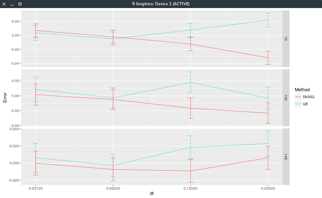
I stumbled recently upon a new Heston discretisation scheme, in the spirit of Alfonsi, not more complex and more accurate.
My first attempt at coding the scheme resulted in a miserable failure even though the described algorithm looked
not too difficult. I started wondering if the paper, from a little known Lithuanian mathematical journal, was any good.
Still, the math in it is very well written, with a great emphasis on the settings for each proposition.
I decided to simply send an email to Prof. Mackevicius, and got a reply the next day (the internet is wonderful sometimes).
The exchange helped me to find out that the error was not where I was looking. After spending a bit more time on the paper, I discovered there was simply a missing step
in the algorithm.
In between step 3 and step 4, we should have
$$ \bar{x} = \frac{\bar{x}\sigma - \bar{y}\rho}{\sigma^2 \sqrt{1-\rho^2}}$$
$$ \bar{y} = \frac{\bar{y}}{\sigma^2}$$
corresponding to the transformation between equations 4.2 and 4.3 of the 2015 paper.
With the added step, the scheme works well. Even if there is clearly an effort from the authors to make their
very mathematically detailed paper more practical with a description of an algorithm, it looks like I have been the first person
to actually try it.
Jesper Andreasen and Brian Huge propose an arbitrage-free interpolation method
based on a single-step forward Dupire PDE solution in their paper Volatility interpolation.
To do so, they consider a piecewise constant representation of the local volatility in maturity time and strike
where the number of constants matches the number of market option prices.
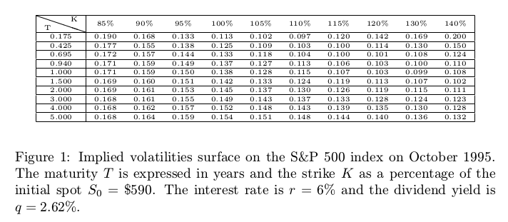
An interesting example that shows some limits to the technique as described in Jesper Andreasen and Brian Huge paper comes from
Nabil Kahale paper on an arbitrage-free interpolation of volatilities.
option volatilities for the SPX500 in October 1995.
Yes, the data is quite old, and as a result, not of so great quality. But it will well illustrate the issue.
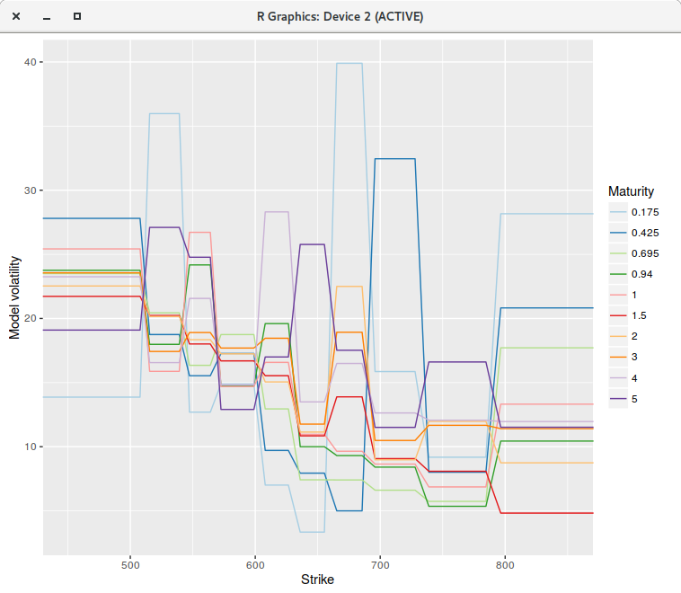
The calibration of the piecewise constant volatilities on a uniform grid of 200 points (on the log-transformed problem) leads to a perfect fit:
the market vols are exactly reproduced by the following piecewise constant vols:
piecewise constant model on a grid of 200 points.
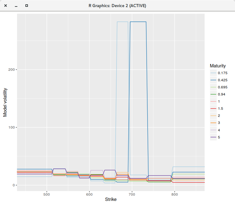
However, if we increase the number of points to 400 or even much more (to 2000 for example), the fit is not perfect anymore, and
some of the piecewise constant vols explode (for the first two maturities), even though there is no arbitrage in the market option prices.
piecewise constant model on a grid of 400 points.
The single step continuous model can not represent the market implied volatilities, while for some reason,
the discrete model with 200 points can. Note that the model vols were capped, otherwise they would explode even higher.
If instead of using a piecewise constant representation, we consider a continuous piecewise linear interpolation
(a linear spline with flat extrapolation), where each node falls on the grid point closest market strike, the calibration
becomes stable regardless of the number of grid points.
piecewise linear model on a grid of 400 points.
The RMSE is back to be close to machine epsilon. As a side effect the Levenberg-Marquardt minimization takes much less iterations to converge, either with 200 or 400 points when compared to the piecewise constant model,
likely because the objective function derivatives are smoother.
In the most favorable case for the piecewise constant model,
the minimization with the linear model requires about 40% less iterations.
We could also interpolate with a cubic spline, as long as we make sure that the volatility does not go below zero, for example by imposing a limit on the derivative values.
Overall, this raises questions on the interest of the numerically much more complex continuous time version of the piecewise-constant model
as described in Filling the gaps by Alex Lipton and Artur Sepp: a piecewise constant representation is too restrictive.
We will assume zero interest rates and no dividends on the asset \(S\) for clarity.
The results can be easily generalized to the case with non-zero interest rates and dividends.
Under those assumptions, the Black-Scholes PDE is:
$$ \frac{\partial V}{\partial t} + \frac{1}{2}\sigma^2 S^2 \frac{\partial^2 V}{\partial S^2} = 0.$$
An implicit Euler discretisation on a uniform grid in \(S\) of width \(h\) with linear boundary conditions (zero Gamma) leads to:
$$ V^{k+1}_i - V^{k}_i = \frac{1}{2}\sigma^2 \Delta t S_i^2 \frac{V^{k}_{i+1}-2V^k_{i}+V^{k}_{i-1}}{h^2}.$$
for \(i=1,…,m-1\) with boundaries
$$ V^{k+1}_i - V^{k}_i = 0.$$
for \(i=0,m\).
This forms a linear system \( M \cdot V^k = V^{k+1} \) with \(M\) is a tridiagonal matrix where each of its rows sums to 1 exactly.
Furthermore, the payoff corresponding to the forward price \(V_i = S_i\) is exactly preserved as well by such a system as the discretized second derivative will be exactly zero.
The scheme can be seen as preserving the zero-th and first moments.
As a consequence, by linearity, the put-call parity relationship will hold exactly (note that in between nodes, any interpolation used should also be consistent with the put-call parity for the result to be more general).
This result stays true for a non-uniform discretisation, and with other finite difference schemes as shown in this paper.
It is common to consider the log-transformed problem in \(X = \ln(S)\) as the diffusion is constant then, and a uniform grid much more adapted to the process.
$$ \frac{\partial V}{\partial t} + \frac{1}{2}\sigma^2 \frac{\partial^2 V}{\partial X^2}-\frac{1}{2}\sigma^2 \frac{\partial V}{\partial X} = 0.$$
An implicit Euler discretisation on a uniform grid in \(X\) of width \(h\) with linear boundary conditions (zero Gamma in \(S\) ) leads to:
$$ V^{k+1}_i - V^{k}_i = \frac{1}{2}\sigma^2 \Delta t \frac{V^{k}_{i+1}-2V^k_{i}+V^{k}_{i-1}}{h^2}-\frac{1}{2}\sigma^2 \Delta t \frac{V^{k}_{i+1}-V^{k}_{i-1}}{2h}.$$
for \(i=1,…,m-1\) with boundaries
$$ V^{k+1}_i - V^{k}_i = 0.$$
for \(i=0,m\).
Such a scheme will not preserve the forward price anymore. This is because now, the forward price is \(V_i = e^{X_i}\). In particular, it is not linear in \(X\).
It is possible to preserve the forward by changing slightly the diffusion coefficient, very much as in the exponential fitting idea. The difference is that, here, we are not interested
in handling a large drift (when compared to the diffusion) without oscillations, but merely to preserve the forward exactly.
We want the adjusted volatility \(\bar{\sigma}\) to solve
$$\frac{1}{2}\bar{\sigma}^2 \frac{e^{h}-2+e^{-h}}{h^2}-\frac{1}{2}\sigma^2 \frac{e^{h}-e^{-h}}{2h}=0.$$
Note that the discretised drift does not change, only the discretised diffusion term. The solution is:
$$\bar{\sigma}^2 = \frac{\sigma^2 h}{2} \coth\left(\frac{h}{2} \right) .$$
This needs to be applied only for \(i=1,…,m-1\).
This is actually the same adjustment as the exponential fitting technique with a drift of zero. For a non-zero drift, the two adjustments would differ, as the exact forward adjustment will stay the same, along with an adjusted discrete drift.
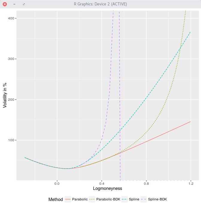
We have seen earlier that a simple parabola allows to capture the smile of AAPL 1m options surprisingly well. For very high and very low strikes,
the parabola does not obey Lee’s moments formula (the behavior in the wings needs to be at most linear in variance/log-moneyness).
Extrapolating the volatility smile in the low or high strikes in a smooth \(C^2\) fashion is however not easy.
A surprisingly popular so called “arbitrage-free”
method is the extrapolation of Benaim, Dodgson and Kainth developed to remedy the negative density of SABR in interest rates as
well as to give more control over the wings.
The call options prices (right wing) are extrapolated as:
$$
C(K) = \frac{1}{K^\nu} e^{a_R + \frac{b_R}{K} + \frac{c_R}{K^2}} \text{.}
$$
\(C^2\) continuity conditions for the right wing at strike \(K_R\) lead to:
$$
c_R =\frac{{C’}_R}{C_R}K_{R}^3+ \frac{1}{2}K_{R}^2 \left(K_{R}^2 \left(- \frac{{C’}_{R}^{2}}{C_{R}^2}+ \frac{{C’’}_R}{C_R}\right) + \nu \right)\text{,} \
$$
$$
b_R = - \frac{{C’}_R}{C_R} K_R^2 - \nu K_R-2 \frac{c_R}{K_R}\text{,}\
$$
$$
a_R = \log(C_R)+ \nu \log(K_R) - \frac{b_R}{K_R} - \frac{c_R}{K_{R}^2}\text{.}
$$
The \( \ nu \) parameters allow to adjust the shape of the extrapolation.
Unfortunately it does not really work for equities.
Very often, the extrapolation will explode, which is what we wanted to avoid in the first place. We illustrate it here on
our best fit parabola of the AAPL 1m options:
BDK explodes on AAPL 1m options.
The \( \nu\) parameter does not help either.
Update Dec 5 2016
Here are details about call option price, slope, curvature:
The strike cutoff is \(K_R=115.00001307390328\). For the parabola,
For the least squares spline,
$$\begin{align}
C(K_R)&=0.03892674300426042,\\
C’(K_R)&=-0.00171386452499034,\\
C’’(K_R)&=0.0007835686926501496.
\end{align}$$
which results in
$$a_R=131.894286, b_R=-26839.217814, c_R=1550285.706087.$$
In finance, and also in science, the Mersenne-Twister is the de-factor pseudo-random number generator (PRNG) for Monte-Carlo simulations.
By the way, there is a recent 64-bit maximally equidistributed version called MEMT19937 with 53-bit double precision floating point numbers in mind.
Historicaly, counter-based PRNGs based on cryptographic standards such as AES
were historically slow, which motivated the development of sequential PRNGs with good statistical properties,
yet not cryptographically strong like the Mersenne Twister for Monte-Carlo simulations.
The randomness of AES is of vital importance to its security making the use of the AES128 encryption algorithm as PRNG sound (see Hellekalek & Wegenkittl paper).
Furthermore, D.E. Shaw study shows that AES can be faster than Mersenne-Twister.
In my own simple implementation using the standard library of the Go language,
it was around twice slower than Mersenne-Twister to generate random double precision floats,
which can result in a 5% performance loss for a local volatility simulation.
The relative slowness could be explained by the type of processor used, but it is still competitive for Monte-Carlo use.
The code is extremely simple, with many possible variations around the same idea. Here is mine
Interestingly, the above code was 40% faster with Go 1.7 compared to Go 1.6, which resulted in a local vol Monte-Carlo simulation performance improvement of around 10%.
The stream cipher Salsa20 is another possible candidate to use as counter-based PRNG.
The algorithm has been selected as a Phase 3 design in the 2008 eSTREAM project organised by the European Union ECRYPT network,
whose goal is to identify new stream ciphers suitable for widespread adoption.
It is faster than AES in the absence of specific AES CPU instructions.
Our tests run with a straightforward implementation that does not make use of specific AMD64 instructions
and show the resulting PRNG to be faster than MRG63k3a and only 5% slower than MEMT19937 for local volatility Monte-Carlo simulations, that is the same speed as the above Go AES PRNG.
While it led to sensible results, there does not seem any study yet of its equidistribution properties.
Counter-based PRNGs are parallelizable by nature: if a counter is used as plaintext,
we can generate any point in the sequence at no additional cost by just setting
the counter to the point position in the sequence, the generator is not sequential.
Furthermore, alternate keys can be used to create independent substreams:
the strong cryptographic property will guarantee the statistical independence.
A PRNG based on AES will allow \(2^{128}\) substreams of period \(2^{128}\).
I found back some old notes I had written about the book “Le capital au XXI siecle” from Thomas Piketty. It took me a while to finish that book last summer.
So many journalists have written around Piketty, that I had to buy the book and read it. It turns out that some of the criticism I have read is not really founded once one reads the book, but here are other real obvious criticisms that I suprisingly did not hear.
The best part of the book is probably the introduction. It’s actually not so short and gives a good overall view of the main subjects of the book. But it’s a bit too concise to truely understand the point. Unfortunately as the book progresses, it feels more like someone trying to fill up empty pages than real content. The first half of the first chapter is still interesting, and then we are overwhelmed with too many graphs and even more words to just state the obvious in the graph, or to repeat over and over the same idea. His economic “laws” should really be summarized on one (or two) simple page, there is no need for hundreds of pages to understand them. Banks could learn a bit of basic statistics: Piketty makes the point of not considering only one measure of inequality like the Gini index, very much like banks should not consider only one measure of risk like the VaR.
The title is clever, as it is a direct reference to Marx “The Capital”, but it’s very far from the quality of Marx book. Marx can be wrong about many things, but in each chapter, he presents new ideas, a different way of looking at the problem. There is a real philosophical effort of defining the meaning of words, and there is fascinating analysis of the economic world of the 19th century. I am refering to the first volume, the only one Marx truly wrote.
I hardly understand why Piketty is so popular in the US. I remember how much fun it was to read Adam Smith “The Wealth of Nations”, and again how different perpectives it tries to bring, and it’s no small book either. Piketty is boring, extremely boring to read (except the intro). Maybe the Americans just stopped at the introduction. Likely it has more to do with Piketty being the intellectual defending the same ideas as the very popular Occupy movement (which we somehow don’t hear about so much anymore). Bourdieu was very talented in mixing the right amount of statistics with extremely original views along with a philosophical stance. I expected more from Piketty, an admirer of the likes of Bourdieu.
A much more interesting book would be something like a spiced up introduction to this book. One main leitmotiv is the fact that the 21st century will not look like the 20th century, but maybe more like the 19th century. Why wouldn’t the 21st century look like the 21st century, that is different from the 20th and the 19th century? Still, where Picketty is interesting is in the fact that there is something to learn from the 19th century economics, and something to unlearn from the 20th century economics which might be too prevalent today.
Last year, I was kindly invited at the workshop on Models and Numerics in Financial Mathematics at the Lorentz center.
It was surprinsgly interesting on many different levels. Beside the relatively large gap between academia and the industry, which this
workshop was trying to address, one thing that struck me is how difficult it was for people of slightly different specialties to communicate.
It seemed that mathematicians of different countries working on different subjects related to backward stochastic differential equations (BSDEs) would not truly understand each other. I know this is
very subjective, and maybe those mathematicians did not feel this at all. One concrete example is related to the number of regressors needed to solve a BSDE on 10 different variables.
Solving a BSDE on 10 variables for EDF was given as an illustration at the end of an otherwise excellent presentation.
Someone in the audience asked how possibly they could do that in practice since it would involve \(10^{10}\) regression factors. The answer of the speaker was more or less that it was what they do, with no particular trick but with a large computing power, as if \(10^{10}\) was not so big.
At this point I was really wondering why \(10^{10}\). Usually, when we do regressions in some BSDE like algorithm, for example Longstaff-Schwartz for American Monte-Carlo, we don’t consider all the powers of each variables from 0 to 10 as well as their cross products.
We only consider polynomials of degree 10, that is all the cross-combinations that lead to a total degree of 10 or less. On two variables \(X\) and \(Y\), we care about \(1, X, Y, XY, X^2, Y^2\) but we dont care about \(X^2 Y, X Y^2, X^2 Y^2\).
We can count then how many factors would be needed for 10 variables.
We can proceed degree by degree and compute how many ordered ways we can add \(N\) non negative integers to produce the given degree \(D\) for each degree and \(N=10\).
This number is simply \( C^{N+D-1}_{N-1} = C^{N+D-1}_D \) where \(C_k^n \) denotes the binomial coefficient.
If this number is not so obvious, we can proceed step by step as well: for degree 1, there is just \( N \) factors (we assign 1 to one of the variables).
For degree 2, there is \(N\) factors to place the number 2 on each variable, plus \( C^N_2 \) to place (1,1) on the variables. From Pascal triangle, we have \( C^{N+1}_{2} = C^N_2 + C^N_1\).
For degree 3, there is \(N\) factors to place the number 3 on each variable, plus \( C^N_3 \) to place the numbers (1,1,1) on the variables plus \(2C^N_2\) to place (1,2) and (2,1). Applying the Pascal identity twice, we have \( C^{N+2}_{3} = (C^N_1+ C^N_2) + (C^N_2 + C^N_3)\). etc.
Thus the total number of factors for \(N\) variables is
For \(N=10\), the total number of factors is 184756.
Although, the total number of factors is large, it is much less than \(10^{10}\). The surprising fact of the workshop is that there were many very advanced mathematicians in the audience, specialists of BSDEs, and none made a comment to help the presenter.
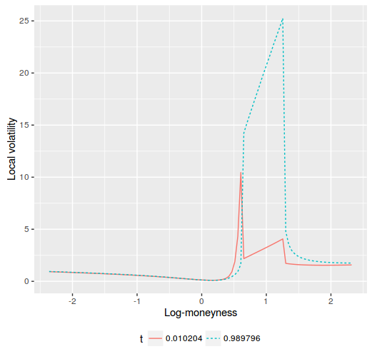
In my previous post, I looked at de-arbitraging volatilities of options of a specific maturity with the shooting method.
In reality it is not so practical. While the local volatility will be continuous at the given expiry \(T\), it won’t be so at the times \( t \lt T \)
because of the interpolation or extrapolation in time. If we consider a single market expiry at time \(T\),
it is standard practice to extrapolate the implied volatility flatly for \(t \lt T\), that is, \(w(y,t) = v_T(y) t\)
where the variance at time \(T\) is defined as \(v_T(y)= \frac{1}{T}w(y,T)\).
Plugging this into the local variance formula leads to
$$\sigma^{\star 2}\left(y, t\right) = \frac{ v_T(y)}{1 - \frac{y}{v_T}\frac{\partial v_T}{\partial y} + \frac{1}{4}\left(-\frac{t^2}{4}-\frac{t}{v_T}+\frac{y^2}{v_T^2}\right)\left(\frac{\partial v_T}{\partial y}\right)^2 + \frac{t}{2}\frac{\partial^{2} v_T}{\partial y^2}}$$
for \(t\leq T\). In particular, for \(t=0\), we have
$$\sigma^{\star 2}\left(y, 0\right) = \frac{ v_T(y)}
{1 - \frac{y}{v_T}\frac{\partial v_T}{\partial y} + \frac{1}{4}\left(\frac{y^2}{v_T^2}\right)\left(\frac{\partial v_T}{\partial y}\right)^2}$$
But the first derivative is not continuous, and jumps at \(y=y_0\) and \(y=y_1\). The local volatility will jump as well around those points. Thus, in practice, the technique can not be used for pricing under local volatility.
jumping local volatility on Axel Vogt example fixed by shooting
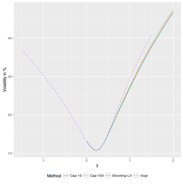
The local volatility stays very high in the original arbitrage region, very much like a capped local volatility would do. It should be then no surprise that in the equivalent implied volatility
is nearly the same as the one stemming from a capped local variance (we imply the smile from the prices of the local volatility PDE).
implied volatility on Axel Vogt example fixed by shooting or by capping
The discontinuity renders the shooting technique useless.
The penalized spline does not have this issue as the resulting local volatility is smooth from \(t=0\) to \(t=T\).