Around 15 years ago, I wrote a small Java applet to try and show the Benham disk effect. Even back then applets were already passé and Flash would have been more appropriate. These days, no browser support Java applets anymore, and very few web users have Java installed. Flash also mostly disappeared. The web canvas is today’s standard allowing to embbed animations in a web page.
This effect shows color perception from a succession of black and white pictures. It is a computer reproduction from the Benham disc with ideas borrowed from "Pour La Science Avril/Juin 2003".
Using a delay between 40 and 60ms, the inner circle should appear red, the one in the middle
blue and the outer one green. When you reverse the rotation direction,
blue and red circles should be inverted.
There are not many blogs on quantitative finance that I read. Blogs are not so popular anymore with the advent of the various social networks (facebook, stackoverflow, google plus, reddit, …). Here is a small list:
Implementing Quantlib: the blog from Luigi Ballabio, which explains many of the design decisions in Quantlib. Very interesting for developer of financial libraries, see for example the fd solvers.
HPC Quantlib from Klaus Spanderen. Yes lots of quantlib blogs, but this one is actually not much focused on quantlib. It goes into great details about some numerical techniques, see for example the analysis of Heston pricing algorithm
Wilmott forums not a blog, but it sometimes (not often) has interesting discussions and can be a good way to connect.
Another way to find out what’s going on in the quantitative finance world is to scan regularly recent papers on arxiv, SSRN or the suggestions of Google scholar.
Unfortunately, in their main formula for non-negativity, they made a typo: the equation (3.3) is not consistent with the equation (3.1): the \( \Delta x_{i-1/2} \) is interverted with \( \Delta x_{i+1/2} \).
It was not obvious to find out which equation was wrong since there is no proof in the paper. Fortunately, the proof is in the reference paper “Monotone piecewise bicubic interpolation” from Carlson and Fritsch and it is clear then that equation (3.1) is the correct one.
Here is a counter example for equation (3.3) for a Hermite cubic spline with natural boundary conditions
In the above example, even though the step size \(\Delta x\) is constant, the error is visible at the last node since then only one inequation apply, and it will be different with the typo.
It is quite annoying to stumble upon such typos, especially when the equations stem from a derived correct paper. We wonder then where are the other typos in the paper and our trust in the equations is greatly weakened. Unfortunately, such mistakes happen to everybody, including myself, and they are rarely caught by reviewers.
Dan Stefanica and Rados Radoicic propose a quite good initial guess in their very recent paper An Explicit Implied Volatility Formula. Their formula is simple, fast to compute and results in an implied volatility guess with a relative error of less than 10%.
It is more robust than the rational fraction from Minquiang Li: his rational fraction is only valid for a fixed range of strikes and maturities. The new approximation is mathematically proved accurate across all strikes and all maturities. There is only the need to be careful in the numerical implementation with the case where the price is very small (a Taylor expansion of the variable C will be useful in this case).
As mentioned in an earlier post, Peter Jäckel solved the real problem by providing the code for a fast, very accurate and robust solver along with his paper Let’s be rational. This new formula used as initial guess to Minquiang Li SOR-TS solver provides an interesting alternative: the resulting code is very simple and efficient. The accuracy, relative or absolute can be set to eventually speedup the calculation.
Below is an example of the performance on a few different cases for strike 150, forward 100, time to maturity 1.0 year and a relative tolerance of 1E-8 using Go 1.8.
Original volatility
Method
Implied Volatility
Time
64%
Jäckel
0.6400000000000002
1005 ns
64%
Rational
0.6495154924570236
72 ns
64%
SR
0.6338265040549524
200 ns
64%
Rational-Li
0.6400000010047917
436 ns
64%
SR-Li
0.6400000001905617
568 ns
16%
Rational
0.1575005551326285
72 ns
16%
SR
0.15117970813645165
200 ns
16%
Jäckel
0.16000000000000025
1323 ns
16%
Rational-Li
0.16000000000219483
714 ns
16%
SR-Li
0.16000000000018844
1030 ns
4%
Rational
0.1528010258201771
72 ns
4%
SR
0.043006234681405076
190 ns
4%
Jäckel
0.03999999999999886
1519 ns
4%
Rational-Li
0.040000000056277685
10235 ns
4%
SR-Li
0.040000000000453895
2405 ns
The case 4% was an example of a particularly challenging setting in a Wilmott forum. It results in a very small call option price (9E-25).
The VIX implied volatilities used to look like a logarithmic function of the strikes. I don’t look at them often, but today, I noticed that the VIX had the start of a smile shape.
1m VIX implied volatilities on March 21, 2017 with strictly positive volume.
Very few strikes trades below the VIX future level (12.9). All of this is likely because the VIX is unusually low: not many people are looking to trade it much lower.
Update March 22: Actually the smile in VIX is not particularly new, it is visible in Jim Gatheral 2013 presentation Joint modeling of SPX and VIX for the short maturities. Interestingly, the issue with SVI is also visible in those slides in the shortest maturity.
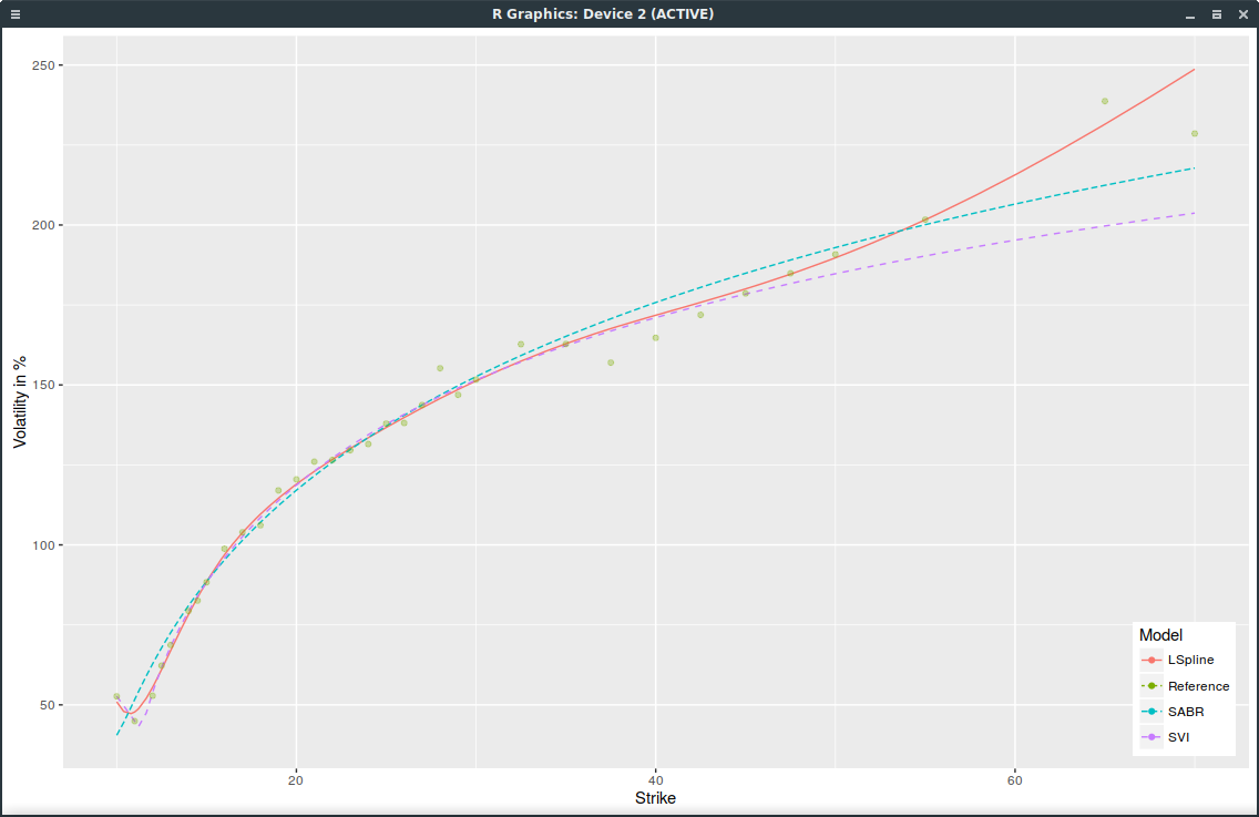
In order to fit the implied volatility smile of equity options, one of the most popular parameterization is Jim Gatheral’s SVI, which I have written about before here.
It turns out that in the current market conditions, SVI does not work well for short maturities. SPX options expiring on March 24, 2017 (one week) offer a good example. I paid attention to include only options with non zero volume, that is options that are actually traded.
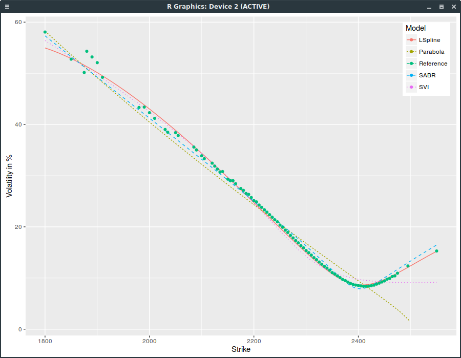
SPXW implied volatilities on March 16, 2017 with strictly positive volume.
SVI does not fit well near the money (the SPX index is at 2385) and has an obviously wrong right wing. This is not due to the choice of weights used for the calibration (I used the volume as weight; equal weights would be even worse). Interestingly, SABR (with beta=1) does much better, even though it has two less parameters than SVI. Also a simple least squares parabola here does not work at all as it ends up fitting only the left wing.
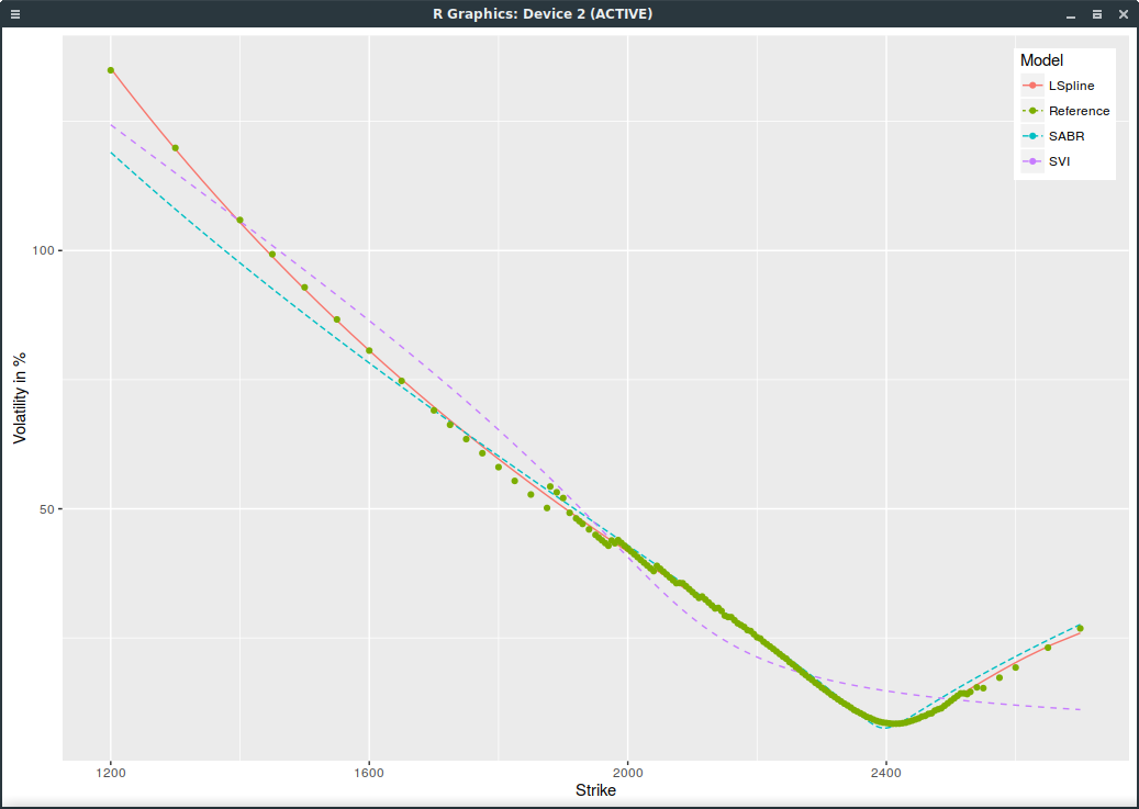
If we include all options with non zero open interest and use ask/(bid-ask) weights, SVI is even worse:
SPXW implied volatilities on March 16, 2017 with strictly positive open interest.
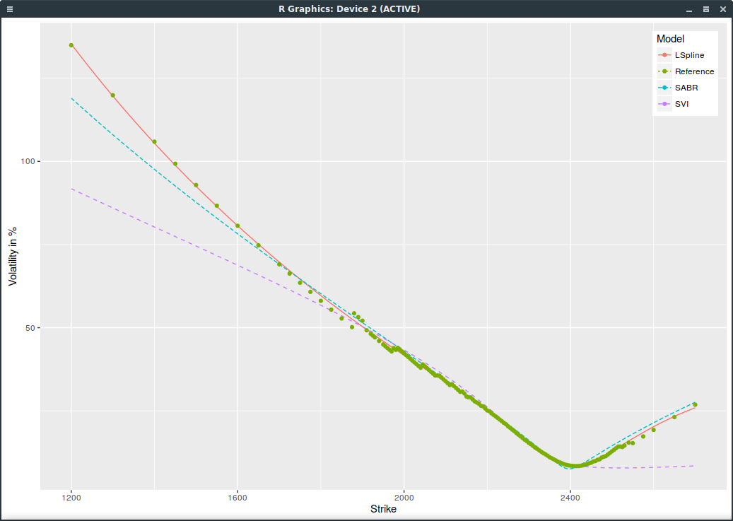
We can do a bit better with SVI by squaring the weights and it shows the problem of SVI more clearly:
SPXW implied volatilities on March 16, 2017 with strictly positive open interest and SVI weights squared.
These days, the VIX index is particularly low. Today, it is at 11.32. Usually, a low VIX translates to growing stocks as investors are confident in a low volatility environment. The catch with those extremely low ATM vols, is that the curvature is more pronounced, and so people are not so confident after all.
The new Heston discretisation scheme I wrote about a few weeks ago makes use
a discrete random variable matching the first five moments of the normal distribution instead of the usual
normally distributed random variable, computed via the inverse cumulative distribution function. Their discrete random
variable is:
$$\xi = \sqrt{1-\frac{\sqrt{6}}{3}} \quad \text{ if } U_1 < 3,,$$
$$ \xi =-\sqrt{1-\frac{\sqrt{6}}{3}} \quad \text{ if } U_1 > 4,,$$
$$\xi = \sqrt{1+\sqrt{6}} \quad \text{ if } U_1 = 3,,$$
$$\xi = -\sqrt{1+\sqrt{6}} \quad \text{ if } U_1 = 4,,$$
with \(U_1 \in \{0,1,…,7\}\)
The advantage of the discrete variable is that it is much faster to generate. But there are some interesting
side-effects. The first clue I found is a loss of accuracy on forward-start vanilla options.
By accident, I found a much more interesting side-effect: you can not use the Brownian-Bridge variance reduction
on the discrete random variable. This is very well illustrated by the case
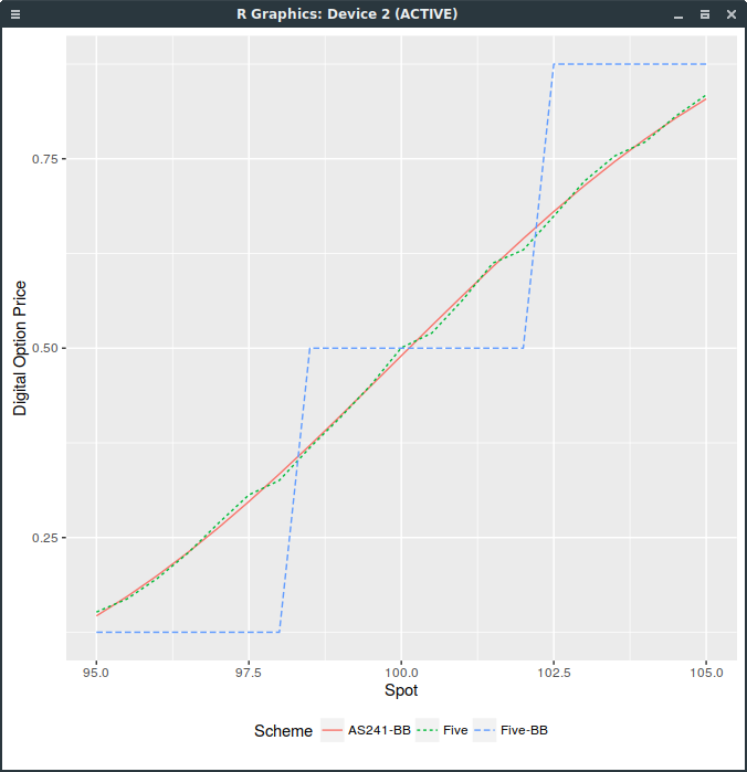
of a digital option in the Black model, for example with volatility 10% and a 3 months maturity, zero interest rate and dividends. For the following graph,
I use 16000 Sobol paths composed of 100 time-steps.
Digital Call price with different random variables.
The “-BB” suffix stands for the Brownian-Bridge path construction, “Five” for five moments discrete variable
and “AS241” for the inverse cumulative distribution function (continuous approach). As you can see,
the price is discrete, and follows directly from the discrete distribution.
The use of any random number generator with a large enough number of paths would lead to the same conclusion.
This is because with the Brownian-Bridge technique, the last point in the path, corresponding to the maturity,
is sampled first, and the other path points are then completed inside from the first and last points.
But the digital option depends only on the value of the path at maturity, that is, on this last point.
As this point corresponds follows our discrete distribution, the price of the digital option is a step function.
In contrast, for the incremental path construction, each point is computed from the previous point.
The last point will thus include the variation of all points in the path, which will be very close to normal, even with a discrete distribution per point.
The take-out to price more exotic derivatives (including forward-start options) with discrete random variables
and the incremental path construction, is that several intermediate time-steps (between payoff observations)
are a must-have with discrete random variables, however small is the original time-step size.
Furthermore, one can notice the discrete staircase even with a relavely small time-step for example of 1/32 (meaning 8 intermediate time-steps in
our digital option example). I suppose this is a direct consequence of the digital payoff discontinuity. In Talay
“Efficient numerical schemes for the approximation of expectations of functionals of the solution of a SDE, and applications” (which you can
read by adding .sci-hub.cc to the URL host name), second order convergence
is proven only if the payoff function and its derivatives up to order 6 are continuous. There is something natural
that a discrete random variable imposes continuity conditions on the payoff, not necessary with a continuous,
smooth random variable: either the payoff or the distribution needs to be smooth.
This is a note for those who want to setup a Samsung wireless printer under Linux. It is quite simple,
this forum post helped me, the actual useful steps on Fedora 25 are:
download tar.gz linux driver from Samsung website. As root, unpack & install:
tar xvzf SamsungPrinterInstaller.tar.gz
cd uld
./install.sh
in the printer menu, lookup for the wireless key (8 digits),
connect to the printer Wifi network with a computer using the wireless key,
A couple weeks ago, I wrote about a new Heston discretisation scheme which was at least as accurate as Andersen QE scheme and faster, called DVSS2.
It turns out that it does not behave very well on the following Vanilla forward start option example (which is quite benign).
The Heston parameters comes from a calibration to the market and are
On a standard vanilla option, DVSS2 behaves as advertised in the paper but not on a forward-start option
with forward start date at \(T_1=\frac{7}{8}\) (relatively close to the maturity).
A forward start call option will pay \(\max(S(T)-k S(T_1),0)\).
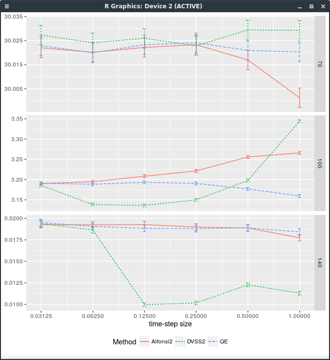
This is particularly visible on the following graph of the price against
the time-step size (1,1/2,1/4,1/8,1/16,1/32), for strikes 100% and 140% (it works well for strike=70%)
where 32 time-steps are necessary.
Forward start Call price with different discretization schemes.
It would appear that the forward dynamic is sometimes poorly captured by the DVSS2 scheme.
This makes DVSS2 not competitive in practice compared to Andersen’s QE or even Alfonsi as it can not be trusted
for a time step larger than 1/32.
Note that I insert an extra step at 7/8 for time step sizes greater or equal than 1/4: a time-step size of 1 corresponds in reality
to two time-steps respectively of size 7/8 and 1/8.
The error is actually because the log-asset process is sampled using a discrete random variables that matches
the first 5 moments of the normal distribution. The so-called step 5 of the algorithm specifies:
$$\hat{X} := \bar{x} + \xi \sqrt{\frac{1}{2}(\bar{y}+\hat{Y})h}$$
The notation is quite specific to the paper, what you need to know is that \(\hat{X}\) corresponds to the log-asset process
while \(\hat{Y}\) corresponds to the stochastic volatility process and \(\xi\) is the infamous discrete random variable.
In reality, there is no good reason to use a discrete random variable beside lowering the computational cost.
And it is obviously detrimental in the limit case where the volatility is deterministic (Black-Scholes case) as then
the log-process will only match the first 5 moments of the normal distribution, while it should be exactly normal.
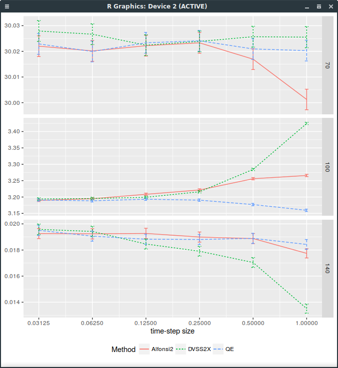
Replacing \(\xi\) by a standard normally distributed random variable is enough to fix DVSS2. Note
that it could also be discretized like the QE scheme, using a Broadie-Kaya interpolation scheme.
Forward start Call price with different discretization schemes. DVSS2X denotes here the scheme with continuous normal random variable.
The problem is that then, it is not faster than QE anymore. So it is not clear why it would be preferable.
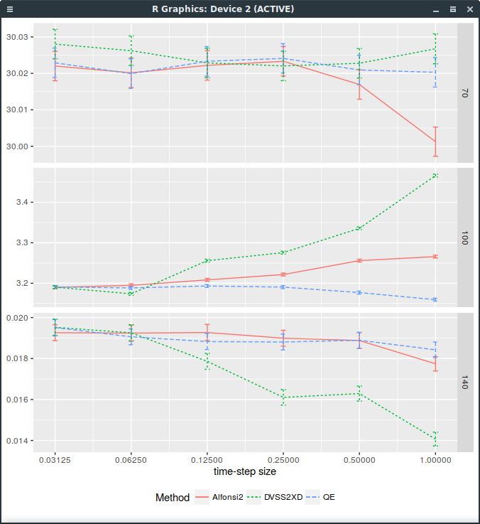
A discrete distribution matching the first 9 moments of the normal distribution
I then tried to see if matching more moments with a discrete distribution would help. More than 8 bits
are available when generating a uniform random double precision number (as it is represented by 53 bits).
The game is then to find nodes so that the distribution with discrete probabilities in i/256 with some interger i
match the moments of the normal distribution. It is a non linear problem unfortunately, but I found a solution
for the probabilities
While this helps a bit for small steps as shown on the following graph, it is far from good:
Forward start Call price with different discretization schemes. DVSS2X denotes here the scheme with discrete random variable matching the first 9 moments of the normal distribution.
The gnome shell has been crashing on me more regularly lately.
XFCE is a good and fast more tradional desktop, but, from past experiences,
it does not play well with power management if you only install it via
dnf install @xfce-desktop-environment
My typical experience is a black screen after resuming from suspend (sometimes, not always), or hibernate (always) and
most of the time I end up just rebooting. It turns out this is all caused by the interaction between the gdm login daemon and xfce. Moving
to the lightdm login daemon instead fixes those issues for Fedora 25: