A new scheme for Heston - Part 2
A couple weeks ago, I wrote about a new Heston discretisation scheme which was at least as accurate as Andersen QE scheme and faster, called DVSS2.
It turns out that it does not behave very well on the following Vanilla forward start option example (which is quite benign). The Heston parameters comes from a calibration to the market and are
$$v_0= 0.0718, \kappa= 1.542, \theta= 0.0762, \sigma= 0.582, \rho= -0.352$$
with a maturity of one year.
On a standard vanilla option, DVSS2 behaves as advertised in the paper but not on a forward-start option
with forward start date at \(T_1=\frac{7}{8}\) (relatively close to the maturity).
A forward start call option will pay \(\max(S(T)-k S(T_1),0)\).
This is particularly visible on the following graph of the price against
the time-step size (1,1/2,1/4,1/8,1/16,1/32), for strikes 100% and 140% (it works well for strike=70%)
where 32 time-steps are necessary.
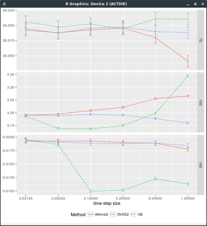
Forward start Call price with different discretization schemes.
It would appear that the forward dynamic is sometimes poorly captured by the DVSS2 scheme. This makes DVSS2 not competitive in practice compared to Andersen’s QE or even Alfonsi as it can not be trusted for a time step larger than 1/32. Note that I insert an extra step at 7/8 for time step sizes greater or equal than 1/4: a time-step size of 1 corresponds in reality to two time-steps respectively of size 7/8 and 1/8.
The error is actually because the log-asset process is sampled using a discrete random variables that matches the first 5 moments of the normal distribution. The so-called step 5 of the algorithm specifies: $$\hat{X} := \bar{x} + \xi \sqrt{\frac{1}{2}(\bar{y}+\hat{Y})h}$$ The notation is quite specific to the paper, what you need to know is that \(\hat{X}\) corresponds to the log-asset process while \(\hat{Y}\) corresponds to the stochastic volatility process and \(\xi\) is the infamous discrete random variable.
In reality, there is no good reason to use a discrete random variable beside lowering the computational cost. And it is obviously detrimental in the limit case where the volatility is deterministic (Black-Scholes case) as then the log-process will only match the first 5 moments of the normal distribution, while it should be exactly normal.
Replacing \(\xi\) by a standard normally distributed random variable is enough to fix DVSS2. Note
that it could also be discretized like the QE scheme, using a Broadie-Kaya interpolation scheme.
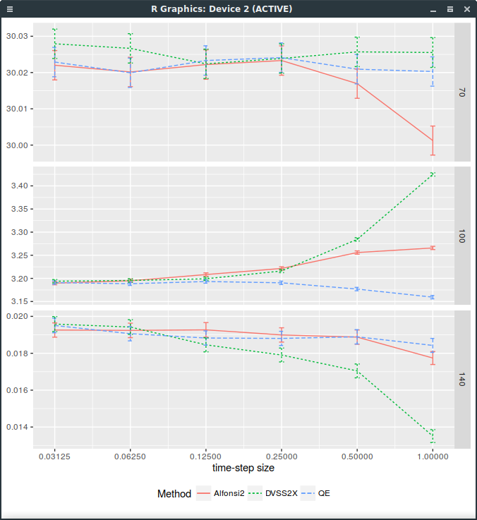
Forward start Call price with different discretization schemes. DVSS2X denotes here the scheme with continuous normal random variable.
The problem is that then, it is not faster than QE anymore. So it is not clear why it would be preferable.
A discrete distribution matching the first 9 moments of the normal distribution
I then tried to see if matching more moments with a discrete distribution would help. More than 8 bits are available when generating a uniform random double precision number (as it is represented by 53 bits). The game is then to find nodes so that the distribution with discrete probabilities in i/256 with some interger i match the moments of the normal distribution. It is a non linear problem unfortunately, but I found a solution for the probabilities
1/256, 1/256, 32/256, 94/256, 94/256, 32/256, 1/256, 1/256-3.1348958252117543, -2.6510063991157273, -1.6397086267587215, -0.5168230803049496, 0.5168230803049496, 1.6397086267587215, 2.6510063991157273, 3.1348958252117543While this helps a bit for small steps as shown on the following graph, it is far from good:
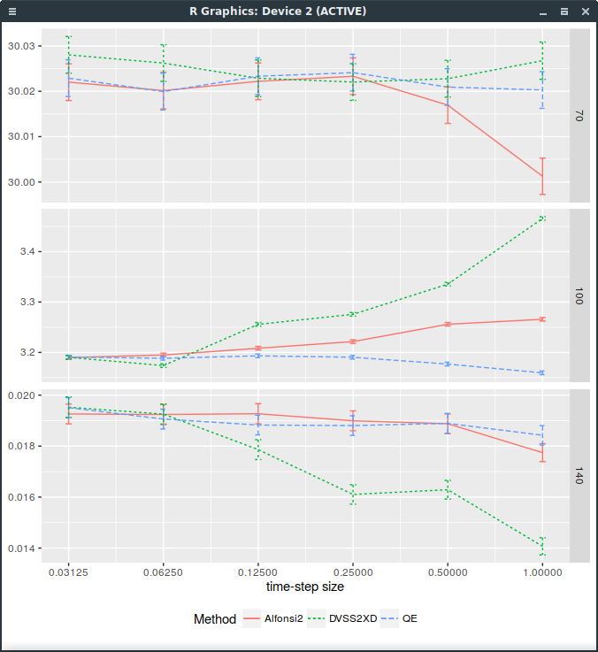
Forward start Call price with different discretization schemes. DVSS2X denotes here the scheme with discrete random variable matching the first 9 moments of the normal distribution.