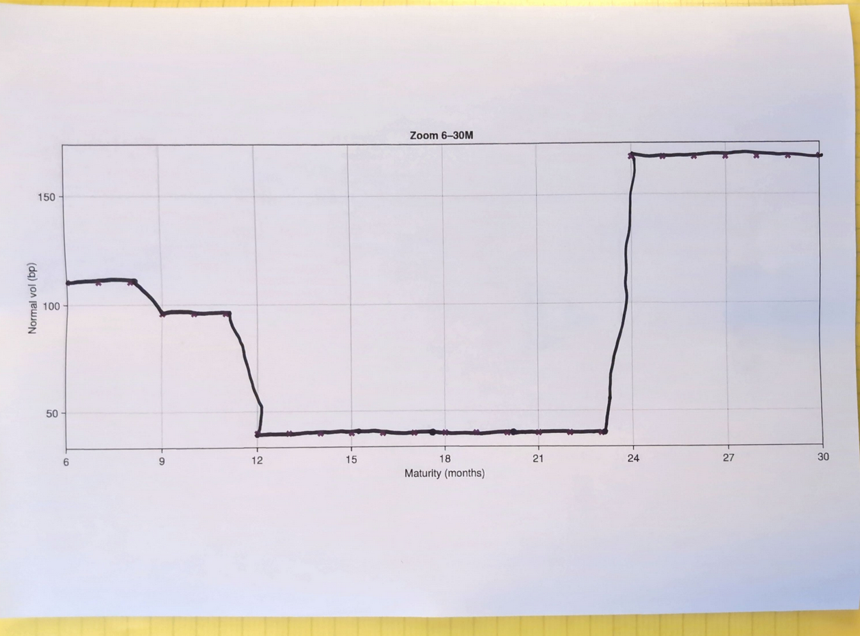
You may or may not have heard that a piecewise-linear interpolation of caplet vols is not stable, it leads to oscillations in the caplet stripping procedure (implying caplet volatilities from cap vol market quotes). And many revert to piecewise-constant interpolation as a consequence.
Several years ago, such a case was brought upon myself and I thought at the time that maybe if we used knots at mid-points it would be more stable as it would balance out the weights in the matrix representation, similarly to what is shown in the book A Practical Guide To Splines, which I particularly enjoyed. I also believed that we must be able to do better than piecewise-constant, which has discontinuities in time, and could thus be problematic for any Theta related measure (sensitivity to time).
During week-ends and off work hours, with my wife wondering what I was spending my time on, I only recently took the time to look at an example of oscillating caplet vols in more details. This led me to many different very interesting paths:
The idea of knots at mid-points indeed works.
The root cause was actually some outliers quotes (although piecewise linear on caplet maturities is not so stable - I explain why). There are ways to filter those out.
Cubic splines also suffer from moderate oscillations when used at caplet maturities vs mid-points.
The piecewise-constant bootstrap stripping is compatible with some piecewise-linear or piecewise-smooth representations.
Gary came up with a direct stripping method based on interpolating prices, which I refined to interpolate time values instead.
The representation with time-values gives immediate clues about arbitrageable quotes (no-arbitrage conditions).
I even asked my children to interpolate bootstrapped caplet volatilities:
Proof that a child does not use piecewise-constant interpolation.
It’s really a joint analysis with Gary Kennedy and this is all detailed in the preprint A Practical Guide to Strip Caplet Volatilities with a clear nod to the book of Carl de Boor. I give code in Java here that allows reproducing some of the results presented (not for production, may contain errors).
Now, the quant bible from Andersen and Piterbarg does not really discuss such stripping methods, which aim at reproducing nearly exactly the market quotes of caps. Instead, it presents a SABR-like fitting procedure in Section 16.2, which is more consistent with the volatility smile at given maturities, but will not match market (or external preprocessed) quotes that well. This reduces the chances of arbitrages in the strike dimension, while I focus only on the maturity dimension (and the caplet vols in the strike dimension may look awkward).
On noisy quotes, the SABR fitting is the better approach. However, nearly exact caplet stripping is very often used in various banking systems.
I have been looking at various techniques for cliquet pricing with a focus on the Heston model. The obvious way is to use Monte-Carlo. Can we do better?
The difficulty of the somewhat simple contract I was looking at is the presence of a global floor, without a local floor, but with a local cap. The payoff reads
\( max(0, min(C, \sum_{i=1}^n \frac{S(t_i)-S(t_{i-1})}{S(t_{i-1})})) \)
where 0 is the global floor, and C is the local cap.
Without global floor, it is just a series of forward starting options and can be easily priced with Heston through a simple Fourier based formula (e.g., the COS method).
With global floor, the option becomes more strongly path-dependent. In a Black-Scholes settings, it all simplifies and pricing it is not so difficult (there are several papers on this, I somewhat wonder if one could not apply the Jamshidian trick as well).
In the tests, N is typically around 1000, so this means a million steps to compute the integral, for evaluating the characteristic function on a single u, and we need N times that. Furthermore, the paper omits any interest rate or dividend yield. Adding those means having to compute a different characteristic function for each period of the cliquet. One can decently wonder then if this is really faster than Monte-Carlo given that the accuracy is not that great either as per Table 1 of that paper.
There is some newer paper on the PROJ method combined with CTMC, it looks very complex to implement, and there are some similar equations as in Deng, so one can wonder if it is not as slow (but it does handle Heston, through a continuous Markov chain approximation).
Finally I found an older paper from Peter den Iseger and Emölde Oldenkamp:Cliquet Options: Pricing and Greeks in Deterministic and Stochastic Volatility Models. This looks much more promising, it details the Black-Scholes simplification, and uses a fancy Legendre basis to not use too many integration points. Still the Heston implementation seems very heavy handed. The more worrying part is that there is no comparison given at all for Heston, no number. The only provided numbers are for the Black-Scholes setting.
There is also the more classic paper named Numerical Methods and Volatility Models for Valuing Cliquet Options by Windcliff, Forsyth and Vetzal on using finite differencing on the PDE, with two additional variables (one for the previous fixing, one for the running sum). On the 2D Heston PDE, it is maybe competitive with Monte-Carlo, maybe not.
Overall, many papers, but none provide any comparison with Monte-Carlo, which is somewhat surprising. Furthermore one may reduce Monte-Carlo variance using the cliquet without global floor as control variate.
Around 2014, I proposed a few Bachelier implied volatility “solvers”. The first one was inspired by Steven G. Johnson’s Faddeeva package for the complex error function: it used a piecewise Chebyshev polynomial representation to have a near machine accurate representation of the Bachelier implied volatility. Why did I put “solver” in quotes? Because the problem can be reduced to a 1D function representation (as originally shown by Choi, Kim and Kwak in 2009). Then, I was encouraged by Gary Kennedy to find a simpler rational function approximation, I used 3 or 4 rational functions to cover the full range of the Bachelier implied volatility function.
Recently, I decided to revisit a little bit the idea, using simpler transformations for some zones to make the solver even faster (and slightly more accurate). Compared to Peter Jäckel’s Implied Normal Volatility solver, it is more than twice as fast. This is because there is a correction step involving the normal density function in P.J.’s solver. Interestingly, testing out initially Quantlib’s implementation gave me the impression it wasn’t so accurate. There may be something wrong there as a direct port of P.J. algo to Rust or Java was very accurate.
Relative error in Bachelier implied volatility as a function of |d|=|K-F|/(sigma*sqrt(T)) when evaluated fully in 64-bit arithmetic.
The paper on the new LFK2026 Normal implied volatlity solver is available at https://arxiv.org/abs/2605.18343 and minimal Java code here. I also give minimal Rust code in the below update (the performance increase is even more significant with Rust).
Update June 16
I have tried two new things:
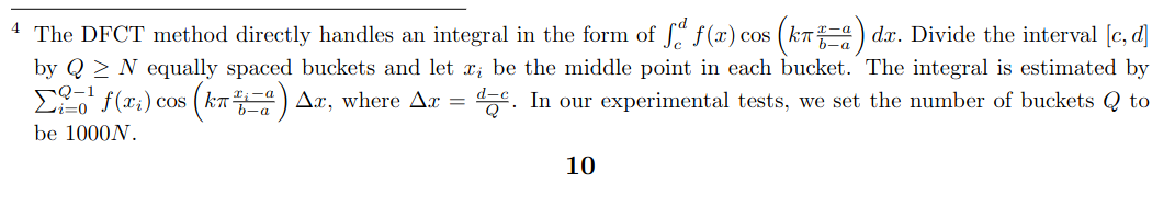
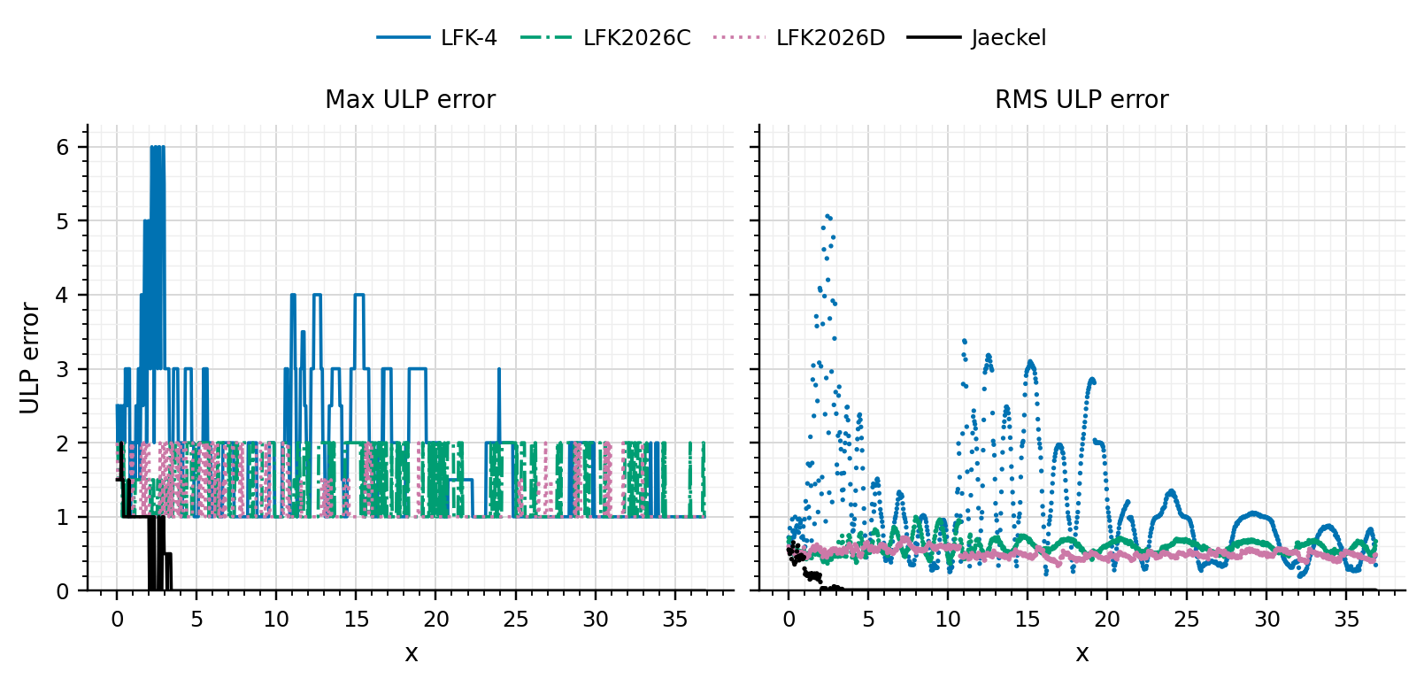
Use of Fused-Multply-Add instructions (FMA) for the Horner evaluation. This speeds up the calculation even more: the new approximations are nearly 3x faster than Jäckel. Another advantage is reduced error overall. This is not so visible in terms of maximum error, the effect is more obvious if we look at the RMSE.
Relative error in Bachelier implied volatility as a function of |d|=|K-F|/(sigma*sqrt(T)) when evaluated fully in 64-bit arithmetic with FMA.
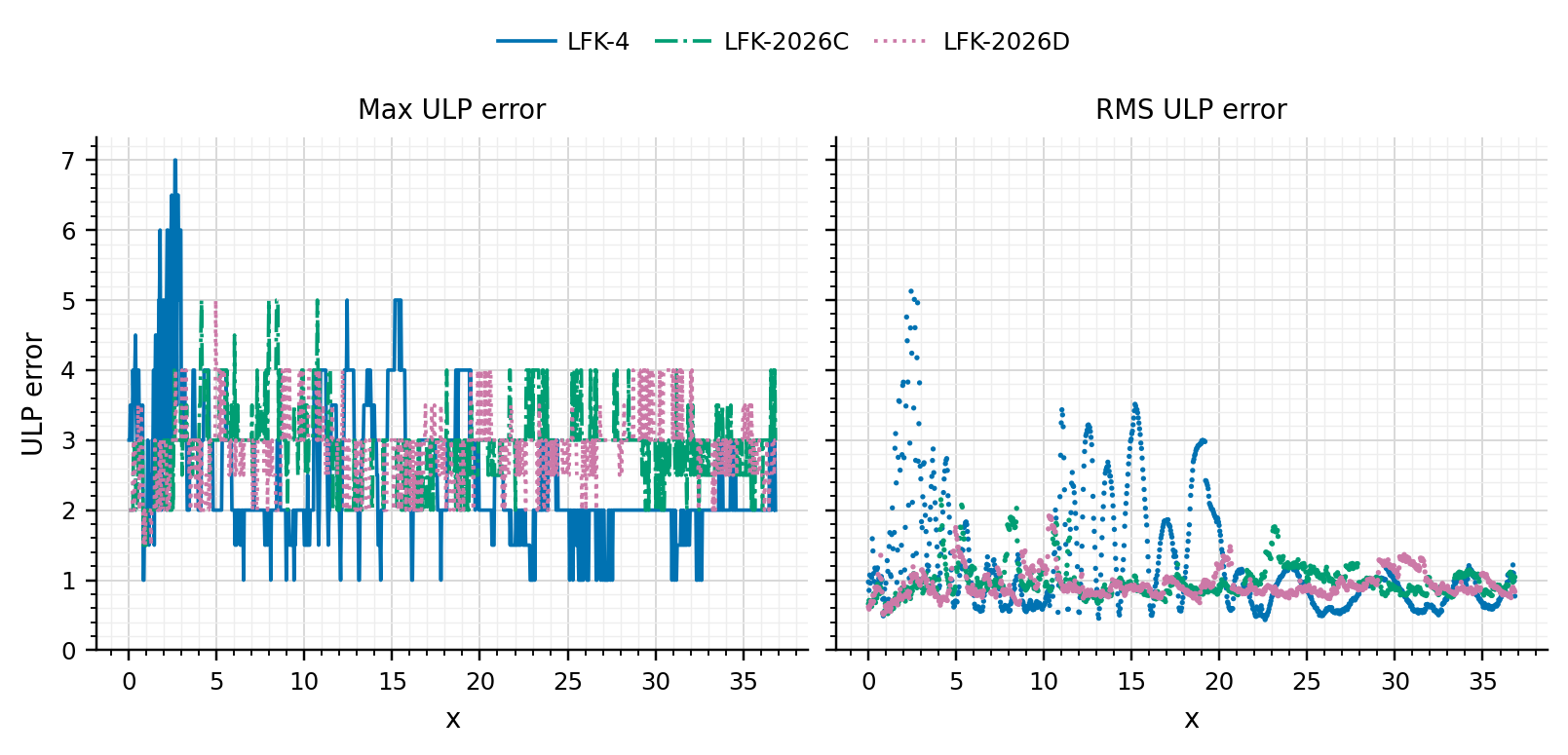
Use of corrected FMA Horner scheme. This allows to gain a few extra (typically two) machine epsilons in accuracy. The cost is decrease in performance (nearly 2x computational cost).
Relative error in Bachelier implied volatility as a function of |d|=|K-F|/(sigma*sqrt(T)) when evaluated fully in 64-bit arithmetic with corrected FMA Horner scheme.
Overall it is quite challenging to increase accuracy further. While it is an interesting problem to look at, it is not necessarily so practical: is this gain of one to three machine epsilons really worth the cost?
Rust code for the LFK solvers and reproduction of the results presented in the paper (instructions in the README.md).
The corresponding forward-normalized OTM-call price is c = B(x, s) / sqrt(ex), with ex = exp(x).
Implementations Compared
Default/current: Jaeckel Region I/II expansions and falls back to the Apache Commons mixed erfc/erfcx formula in the middle region.
Jaeckel acc libm+Commons: the same Jaeckel region-dispatched, included into the temporary harness, using system erf/erfc and the local Apache Commons erfcx.
Jaeckel acc Cody+Cody: the same Jaeckel region-dispatched formula, using Cody erf, erfc, and erfcx from jaeckel = 0.2.0.
Jaeckel acc Johnson+Johnson: the same Jaeckel region-dispatched formula, using Johnson/Faddeeva erf, erfc, and erfcx through errorfunctions = 0.2.0.
Jaeckel acc libm+Cody and Jaeckel acc libm+Johnson: the same formula with system erf/erfc fixed and only erfcx swapped, to isolate the scaled-erfc backend effect.
Jaeckel I/II + pure Commons: Jaeckel Region I/II expansions are kept, but the Region III/middle fallback is replaced by the always-erfcx identity with the local Apache Commons erfcx.
IG statmod upper: the inverse-Gaussian upper-tail representation of the Black beta price, using a scalar Rust port of the CRAN statmod 1.5.2 .pinvgauss mean-one upper-tail log-probability core, with the final log(1-exp(r)) evaluated by a Rust log1mexp helper near cancellation. This is not a full statmod port: it omits R vectorization, NA/Inf handling, finite/infinite-mean special cases, and R’s exact pnorm implementation. The public-wrapper small-CV gamma approximation is also omitted because, under the Black mapping here, it would require dispersion=-2/x < 1e-14, or x < -2e14, far outside the finite Float64x=log(ex) domain. No purpose-built Rust inverse-Gaussian crate was found in cargo search inverse-gaussian / cargo search invgauss; statrs 0.18.0 source also did not contain an inverse-Gaussian/Wald distribution implementation.
Commons erfcx-mixed: the Cody/Jaeckel threshold formula with the local Apache Commons Numbers erfcx port and system erfc.
Cody erfcx-mixed: the same threshold formula using jaeckel = 0.2.0erfcx_cody.
Johnson erfcx-mixed: the same threshold formula using errorfunctions = 0.2.0 Johnson/Faddeeva erfcx.
libm erfc direct: the direct formula above, using system C erfc through FFI. Rust std does not provide erfc or erfcx.
Commons/Cody/Johnson pure-erfcx: the always-erfcx identity 0.5 * exp(-0.5*(h^2+t^2)) * (erfcx(q1) - erfcx(q2)), included to show why the mixed formula avoids some high-volatility tail problems.
Mixed Erfc/Erfcx Fallback Logic
The mixed formula starts from the direct beta-space Black expression:
2B = exp(x/2) * erfc(q1) - exp(-x/2) * erfc(q2)
with
h = x / s
t = s / 2
q1 = -(h + t) / sqrt(2)
q2 = -(h - t) / sqrt(2)
because q1^2 = 0.5 * (h + t)^2, q2^2 = 0.5 * (h - t)^2, and x = h*s = 2*h*t. The mixed implementation uses that identity term by term instead of forcing both terms through one representation.
The branch threshold is Cody’s 0.46875, the same split used by the classic error-function approximations. Arguments below it are kept in the ordinary erfc representation; arguments above it use scaled erfcx so that the small tail probability is not represented as a nearly-underflowed erfc multiplied by a compensating exponential.
if q1 < 0.46875 and q2 < 0.46875:
    2B = exp(x/2) * erfc(q1)
       - exp(-x/2) * erfc(q2)

if q1 < 0.46875 and q2 >= 0.46875:
    2B = exp(x/2) * erfc(q1)
       - exp(-0.5 * (h^2 + t^2)) * erfcx(q2)

if q1 >= 0.46875 and q2 < 0.46875:
    2B = exp(-0.5 * (h^2 + t^2)) * erfcx(q1)
       - exp(-x/2) * erfc(q2)

if q1 >= 0.46875 and q2 >= 0.46875:
    2B = exp(-0.5 * (h^2 + t^2)) * (erfcx(q1) - erfcx(q2))
On the valid Black domain, the third formal case is actually unreachable. Since t = s/2 >= 0,
q2 - q1 = sqrt(2) * t >= 0,
so q1 >= rho implies q2 >= rho as well. The erfcx, erfc branch would require q1 >= rho and q2 < rho at the same time; that would need negative t, not merely positive h = x/s. It is kept in the branch table only as the symmetric algebraic case.
So “mixed” does not mean that erfc is a fallback after erfcx fails. It means each of the two Black terms is routed to the representation that is locally better conditioned. Negative or central arguments stay with erfc, where erfc(q) is order one and cheap. Positive tail arguments switch to erfcx, where the scaled value remains order 1/q and avoids underflow.
This explains two patterns in the tables below. In the low-volatility OTM tail, direct erfc loses many ulps because it subtracts two tiny tail probabilities after ordinary scaling; the mixed erfcx versions are much better. In the high-volatility upper-price window, the pure-erfcx identity is worse because it exposes the cancellation in erfcx(q1) - erfcx(q2) even when ordinary erfc would have kept one side well behaved.
Reference And Local Windows
Reference values are Julia BigFloat at 512-bit precision, rounded back to Float64. ULP error is the positive-Float64 bit distance to that rounded reference. Each window contains 512 consecutive Float64 values in either s or x, with the other coordinate fixed.
id
zone
axis
x
s
central-atm
central
s
-1.000000e-2
2.000000e-1
tiny-near-atm
tiny-near-atm
s
-1.000000e-8
1.000000e-4
erfc-threshold
branch-transition
s
-1.000000e-1
1.364500e-1
moderate-otm
moderate-otm
s
-1.000000e0
5.000000e-1
low-vol-otm
lower-tail
s
-1.000000e-1
2.000000e-2
deep-otm
lower-tail
s
-3.000000e0
7.000000e-1
far-otm
lower-tail
s
-6.000000e0
1.000000e0
high-vol
upper-price
s
-1.000000e-2
1.000000e1
very-high-vol
upper-price
s
-1.000000e0
5.000000e1
near-overflow-vol
upper-price
s
-1.000000e0
7.500000e1
x-central
x-window
x
-1.000000e-2
2.000000e-1
x-lower-tail
x-window
x
-4.000000e0
8.000000e-1
Global Accuracy
backend
samples
invalid
exact_bits
p50
p95
p99
max
max_rel
worst_window
Default/current
6144
0
2301
1
15
24
40
7.4e-15
far-otm
Jaeckel acc libm+Commons
6144
0
2301
1
15
24
40
7.4e-15
far-otm
Jaeckel acc Cody+Cody
6144
0
2291
1
14
22
40
7.4e-15
far-otm
Jaeckel acc Johnson+Johnson
6144
0
2296
1
15
25
42
7.8e-15
far-otm
Jaeckel acc libm+Cody
6144
0
2291
1
14
22
40
7.4e-15
far-otm
Jaeckel acc libm+Johnson
6144
0
2296
1
15
25
42
7.8e-15
far-otm
Jaeckel I/II + pure Commons
6144
0
1277
4
686
1202
1570
2.9e-13
near-overflow-vol
Commons erfcx-mixed
6144
0
1212
5
2823
3019
3068
5.2e-13
tiny-near-atm
IG statmod upper
6144
0
1158
7
6372
6568
7666
1.5e-12
low-vol-otm
Cody erfcx-mixed
6144
0
1180
6
2823
3019
3068
5.2e-13
tiny-near-atm
Johnson erfcx-mixed
6144
0
1161
6
2823
3019
3068
5.2e-13
tiny-near-atm
libm erfc direct
6144
0
1116
10
3049
5952
10329
2.0e-12
low-vol-otm
Commons pure-erfcx
6144
0
255
13
1776
1972
2021
3.4e-13
tiny-near-atm
Cody pure-erfcx
6144
0
174
15
9968
10164
10213
1.7e-12
tiny-near-atm
Johnson pure-erfcx
6144
0
257
19
59120
59316
59365
1.0e-11
tiny-near-atm
The headline is different from the raw erfcx comparison. In the normalized Black formula, the largest errors in these local windows are not the raw negative-erfcx overflow tail. They are tiny near-ATM and low-volatility OTM cancellation zones. The default is much better there because it uses Jaeckel Region I/II expansions before falling back to the mixed erfc/erfcx formula. Once that region-dispatched formula is kept, backend choice barely moves the result: all Jaeckel-accurate variants have global p50 = 1 ulp and max = 40 to 42 ulps on this sample set.
Jaeckel Accurate Backend Sensitivity
The Jaeckel accurate path is not just the mixed formula with a different erfcx. It routes first through:
Region I: asymptotic expansion times the normalized vega. This path is independent of erf, erfc, and erfcx.
Region II: small-t expansion times the normalized vega. This path uses erfcx only in the central y_prime branch; deeper left-tail y_prime is rational.
Region III/middle: the mixed Cody/Jaeckel erfc/erfcx formula described above.
That dispatch is why the special-function backend differences collapse compared with the generic mixed or pure-erfcx formulas.
Selected Jaeckel-accurate rows:
backend
global p50
p95
p99
max
tiny max
low-vol max
erfc-threshold max
far-otm max
Default/current
1
15
24
40
1
17
2
40
Jaeckel acc libm+Commons
1
15
24
40
1
17
2
40
Jaeckel acc Cody+Cody
1
14
22
40
1
17
2
40
Jaeckel acc Johnson+Johnson
1
15
25
42
1
17
2
42
Jaeckel acc libm+Cody
1
14
22
40
1
17
2
40
Jaeckel acc libm+Johnson
1
15
25
42
1
17
2
42
The paired Cody rows match the libm+Cody rows in aggregate, and the paired Johnson rows match the libm+Johnson rows in aggregate. In these windows, the small residual backend sensitivity comes from erfcx, not from swapping the ordinary erf/erfc implementation. Cody is fractionally better than Commons by p95/p99 in the far-OTM-dominated aggregate; Johnson is fractionally worse, with a 42-ulp maximum instead of 40. Those differences are tiny next to the thousands of ulps lost by the non-Jaeckel mixed/direct formulas in the tiny near-ATM and low-vol OTM windows.
Jaeckel I/II With Pure-Erfcx Fallback
A tempting simplification is to keep Jaeckel Regions I and II, but replace the Region III/middle fallback with the pure-erfcx identity:
With Apache Commons erfcx, this is not as accurate as the default (Apache Commons erfc and erfcx with all Jaeckel zones) overall:
backend
global p50
p95
p99
max
tiny max
low-vol max
high-vol max
very-high max
near-overflow max
Default/current
1
15
24
40
1
17
1
0
0
Jaeckel acc libm+Commons
1
15
24
40
1
17
1
0
0
Jaeckel I/II + pure Commons
4
686
1202
1570
1
17
60
745
1570
The simplification keeps the important Region II tiny near-ATM behavior and the Region I/II lower-tail behavior, so those windows match the default. The loss comes from middle/fallback cases, especially the high-volatility upper-price windows. There the pure-erfcx identity exposes cancellation in erfcx(q1) - erfcx(q2), while the mixed fallback keeps the locally better erfc representation for negative or central arguments.
It is not meaningfully faster in this diagnostic either. On the same optimized local-window timing run, the pure fallback row was 24.83 ns/call, compared with 24.80 ns/call for the same included Jaeckel formula with the mixed Commons fallback and 25.07 ns/call for the Default/current path. That difference is inside normal microbenchmark noise, and the generic pure-erfcx kernel was slower than the generic mixed Commons kernel (21.32 vs 19.80 ns/call).
Inverse Gaussian Formula Experiment
For x < 0, the Black beta price can be written as an inverse-Gaussian upper tail. In the statmod mean-one parameterization, let
q = -2x / s^2
dispersion = -2 / x
Y ~ IG(mean = 1, dispersion)
Substituting q=-2x/s^2 and dispersion=-2/x gives the ordinary Black expression in a different parameterization. The temporary Rust harness ports the statmod .pinvgauss core branch for this scalar mean-one upper tail, including its asymptotic right-tail override, and evaluates the normal log tails with the local Apache Commons erfcx support.
One Rust-side numerical improvement was kept: statmod writes the upper-tail combination as a + log1p(-exp(b-a)); the harness uses the equivalent a + log1mexp(b-a), switching to log(-expm1(b-a)) when b-a is close to zero. That slightly reduces cancellation in the tiny near-ATM and low-volatility OTM windows, but it does not change the conclusion.
The one public-wrapper branch that looks relevant at first glance is statmod’s small-CV gamma approximation:
if mean * dispersion < 1e-14:
    pgamma(q, shape=1/(mean*dispersion), scale=(mean*dispersion)*mean)
For this Black identity mean=1 and dispersion=-2/x, so the branch would need x < -2e14. A finite Float64 normalized Black input derived from ex=exp(x)>0 has x >= log(5e-324) ~= -744.44. The gamma approximation therefore cannot trigger on the valid Black domain tested here; implementing it would not change these results.
After installing R, the temporary harness was checked against the actual R code by sourcing the CRAN statmod 1.5.2 R/invgauss.R file. The statmod package was not installed as an R library on this machine, so this is a source-level check of the same public R implementation rather than a namespace-loaded package check. On the 6144 Black-mapped local-window samples, R’s public pinvgauss(..., lower.tail=FALSE, log.p=TRUE) and the literal .pinvgauss core agree exactly in price space, confirming that no wrapper special case is active on this domain.
The remaining Rust-vs-R price differences come from the normal log-tail backend and the final cancellation. Comparing prices directly:
comparison
exact
p50
p95
p99
max
max_rel
worst
Rust log1mexp price vs R pinvgauss
3020
1
648
2406
7348
1.4e-12
low-vol-otm
Rust literal price vs R core literal
4671
0
64
2461
7421
1.4e-12
low-vol-otm
R wrapper vs R core literal price
6144
0
0
0
0
0.0e0
central-atm
R log1mexp core vs R literal price
4115
0
648
648
648
1.1e-13
tiny-near-atm
Against the Julia BigFloat references, literal R/statmod does not improve the Black price accuracy versus the literal Rust port; it lands on the same conclusion as the Rust experiment:
backend/formula
exact
p50
p95
p99
max
max_rel
worst
Rust IG with log1mexp
1158
7
6372
6568
7666
1.5e-12
low-vol-otm
Rust literal statmod
1174
7
7017
7212
7739
1.5e-12
low-vol-otm
R pinvgauss literal statmod
1691
8
7017
7214
7739
1.5e-12
low-vol-otm
R core with log1mexp
1665
8
6373
6570
7666
1.5e-12
low-vol-otm
So R fidelity is good for the relevant scalar statmod formula, and the only measurable Rust-side deviation kept here is the log1mexp substitution. It slightly improves the IG formula relative to literal R/statmod, but the formula remains far less accurate than the Jaeckel Region I/II expansions in the sensitive Black windows.
This representation is not Jaeckel-accurate on the sensitive windows:
backend
global p50
p95
p99
max
tiny max
low-vol max
high-vol max
very-high max
near-overflow max
Default/current
1
15
24
40
1
17
1
0
0
Commons erfcx-mixed
5
2823
3019
3068
3068
593
1
0
0
IG statmod upper
7
6372
6568
7666
6608
7666
1
0
0
The inverse-Gaussian form is fine in the high-volatility upper-price windows, but it is worse than the mixed erfc/erfcx formula in the tiny near-ATM and low-volatility OTM cancellation windows. It is also slower in this scalar Rust port: 63.00 ns/call on the same local-window timing harness, compared with about 25 ns/call for the Jaeckel-dispatched default and about 20 ns/call for the generic Commons mixed formula.
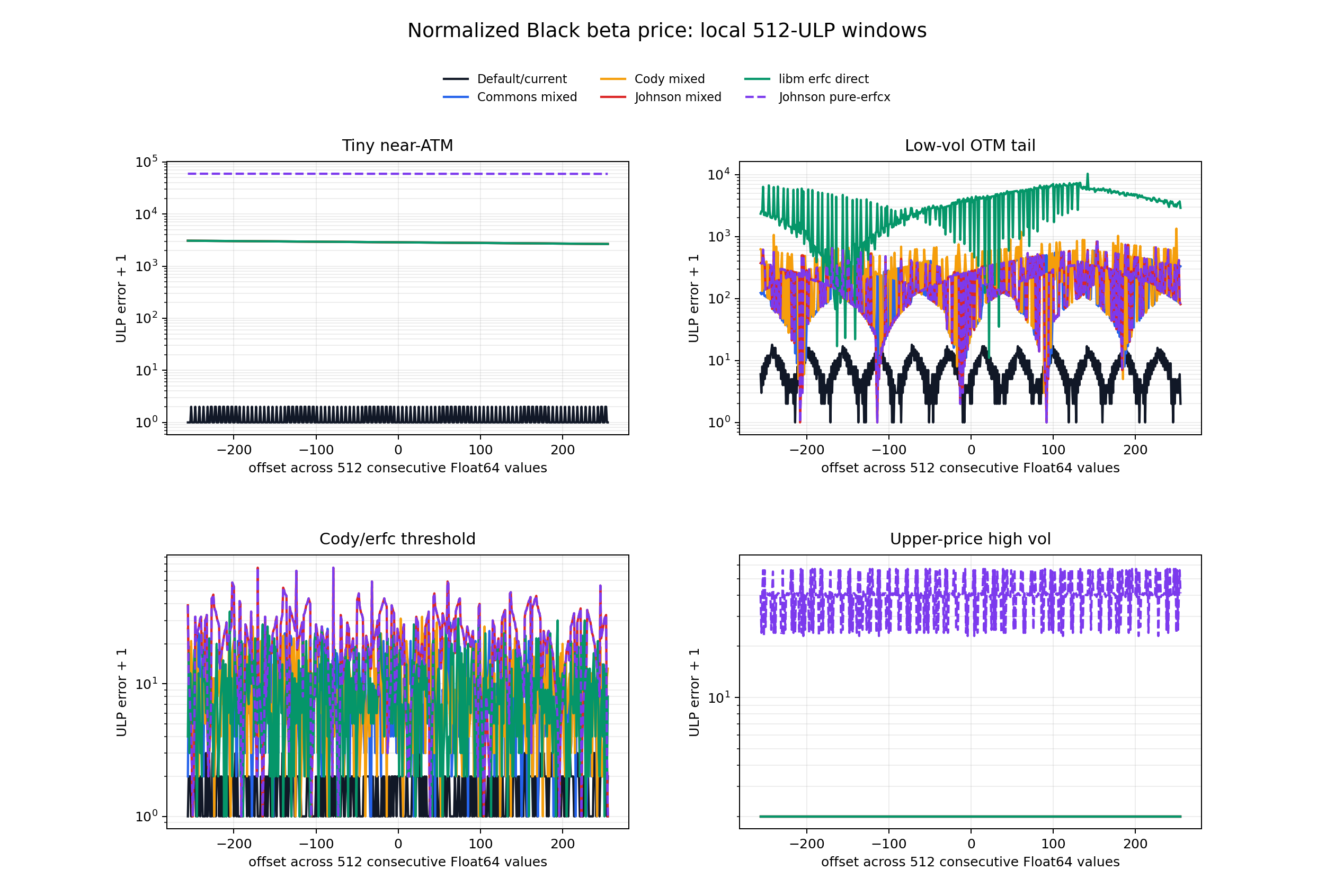
Selected Windows
Black formula local window examples.
Selected 512-ULP window stats:
window = tiny-near-atm
backend
p50
p95
p99
max
Default/current
0
1
1
1
Commons erfcx-mixed
2864
3048
3064
3068
IG statmod upper
6404
6588
6604
6608
Cody erfcx-mixed
2864
3048
3064
3068
Johnson erfcx-mixed
2864
3048
3064
3068
libm erfc direct
2864
3048
3064
3068
Johnson pure-erfcx
59161
59345
59361
59365
window = low-vol-otm
backend
p50
p95
p99
max
Default/current
6
14
16
17
Commons erfcx-mixed
146
429
548
593
IG statmod upper
2299
5108
7130
7666
Cody erfcx-mixed
254
683
885
1345
Johnson erfcx-mixed
180
493
649
831
libm erfc direct
3526
6657
7242
10329
window = erfc-threshold
backend
p50
p95
p99
max
Default/current
1
2
2
2
Commons erfcx-mixed
7
18
23
28
IG statmod upper
9
24
28
32
Cody erfcx-mixed
8
22
28
31
Johnson erfcx-mixed
20
43
57
74
libm erfc direct
7
21
27
34
window = high-vol
backend
p50
p95
p99
max
Default/current
1
1
1
1
Commons erfcx-mixed
1
1
1
1
IG statmod upper
1
1
1
1
Cody erfcx-mixed
1
1
1
1
Johnson erfcx-mixed
1
1
1
1
libm erfc direct
1
1
1
1
Johnson pure-erfcx
39
56
56
57
Interpretation by region:
Tiny near-ATM: backend choice is almost irrelevant for the mixed formula; all mixed/direct forms lose about 3000 ulps. The default Region II expansion stays within 1 ulp.
Low-volatility OTM tail: direct erfc is worst because it subtracts two close tail probabilities. The erfcx-mixed formulas are much better, and Commons is best among the three erfcx backends in this window. The default expansion is better again.
Branch transition: this is where backend differences are visible but modest. Commons and Cody are close; Johnson is weaker but still far from the direct-erfc lower-tail failure.
Upper-price high-volatility: the mixed formula and direct-erfc formula are all within 1 ulp in this window. The pure-erfcx identity is worse because it exposes cancellation/rounding in erfcx(q1) - erfcx(q2) instead of routing negative-side arguments through erfc.
Timing
Timing was measured on the same 6144 local-window samples, best of five passes with 2000 sweeps per pass, using cargo run --release.
backend
ns/call
Default/current
25.07
Jaeckel acc libm+Commons
24.80
Jaeckel acc Cody+Cody
26.55
Jaeckel acc Johnson+Johnson
25.39
Jaeckel acc libm+Cody
23.44
Jaeckel acc libm+Johnson
24.28
Jaeckel I/II + pure Commons
24.83
Commons erfcx-mixed
19.80
IG statmod upper
63.00
Cody erfcx-mixed
17.92
Johnson erfcx-mixed
19.27
libm erfc direct
26.89
Commons pure-erfcx
21.32
Cody pure-erfcx
19.20
Johnson pure-erfcx
19.59
These timings are for the formula kernels on this artificial local-window mix, not for the full IV solvers. The temporary Jaeckel backend rows include a small runtime selector used only by the diagnostic harness. The default is slower than the generic mixed formulas because it does more routing and uses the Region I/II expansion machinery, but the accuracy gain in tiny near-ATM and low-volatility OTM zones is large.
Takeaways
A raw erfcx(x) benchmark overstates the relevance of the negative-erfcx tail for the stable Black price. The mixed formula avoids much of that tail by using erfc on negative-side arguments.
The most important Black-formula accuracy zones here are tiny near-ATM and low-volatility OTM, where formula structure dominates backend choice.
For a generic erfcx-mixed Black formula, Apache Commons is the best of the three tested erfcx backends on the low-vol OTM window, Cody is usually close, and Johnson is somewhat weaker near the branch transition.
For the full Jaeckel accurate formula, all tested backend combinations are essentially tied: global p50 = 1 ulp, max = 40 to 42 ulps, and the sensitive tiny near-ATM window stays within 1 ulp for every backend.
In these sampled windows, swapping Cody or Johnson erf/erfc together with erfcx gives the same aggregate result as keeping libm erf/erfc and swapping only erfcx.
Keeping Jaeckel Regions I/II but using a pure Commons-erfcx fallback is simpler, but not accuracy-equivalent to the default: it matches the default in tiny near-ATM and lower-tail windows, then loses up to 1570 ulps in the high-volatility upper-price fallback region.
The pure-erfcx fallback is not a clear speed win either; in this release-mode diagnostic it was effectively tied with the mixed Jaeckel fallback, while the generic pure-erfcx kernel was slower than the generic mixed Commons kernel.
The inverse-Gaussian/statmod representation is a valid Black formula, but not an accuracy replacement for Jaeckel’s expanded evaluator here: even with a Rust log1mexp cancellation tweak, it loses up to 6608 ulps in the tiny near-ATM window and 7666 ulps in the low-volatility OTM window, and the straightforward scalar port is much slower.
The default remains the accuracy-favored choice because the Jaeckel Region I/II expansions reduce errors from thousands of ulps to tens of ulps or better in the sensitive windows.
References
For the Cody Netlib Slatec codeRational Chebyshev approximations for the error function by W. J. Cody, Math. Comp., 1969, PP. 631-638
For the Apache Commons Number code, this issue description gives a good overview of the implementation, which is a mix of Boost rational functions and Cody rational function to obtain the best accuracy.
Steven G. Johnson mentions in his code the following:
(…) I originally used
an erfcx routine derived from DERFC in SLATEC, but I have
since replaced it with a much faster routine written by
me which uses a combination of continued-fraction expansions
and a lookup table of Chebyshev polynomials. For speed,
I implemented a similar algorithm for Im[w(x)] of real x,
since this comes up frequently in the other error functions.
The use of erfcx instead of direct erfc or CDF in a Black-Scholes implied volatility solver leads to gain in accuracy and performance in general. But which erfcx should we use?
This note compares practical erfcx implementations for Rust implied volatility solvers:
Johnson: Steven G. Johnson’s Faddeeva implementation, as exposed by errorfunctions = 0.2.0, faddeeva-sys = 0.1.0, and Julia SpecialFunctions.erfcx(::Float64)
The Commons-style implementation is a local Rust port of the Apache Commons Numbers/BoostErf approach. It computes the small central region through the local erf rational approximation and uses exp_m1(x*x) to avoid cancellation in exp(x^2) * erfc(x) near zero. For positive inputs it uses several rational subintervals: a central polynomial/rational erf branch, erfc-style rational branches around 0.5..1.5, 1.5..2.5, and 2.5..4, and a rational function taken from Rational Chebyshev approximations for the error function by W. J. Cody, Math. Comp., 1969, PP. 631-638 beyond that. For very large positive x, it returns 1 / (sqrt(pi) * x). For negative x, it uses the reflected form with a split-square exponential, returns Inf below the finite overflow cutoff, and otherwise computes 2 exp(x^2) - erfcx(|x|) in a way that preserves more bits near the overflow boundary.
The Cody implementation used here is the jaeckel crate’s Cody/CALERF-style implementation. It has three main positive-side rational regions: AB for |x| <= 0.46875, CD for 0.46875 < |x| <= 4, and PQ as an asymptotic rational in 1/x^2 for |x| > 4. It uses smoothed exponentials by splitting x onto a 1/16 grid before applying the residual exponential. For negative x, it reflects with erfcx(-x) = 2 exp(x^2) - erfcx(x) and clamps below its XNEG threshold to f64::MAX.
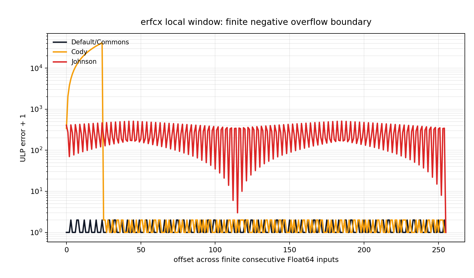
Cody near-overflow spike.
The rare Cody spike in the finite negative overflow-boundary window is not caused by using the wrong rational interval but is deliberate. Cody/CALERF does use the PQ asymptotic rational for the positive |x| > 4 part, but the negative-side fix-up is still the reflected 2 exp(x^2) - erfcx(|x|) form with an XNEG overflow guard. The published IEEE double CALERF constant is the rounded XNEG = -26.628D0; the public Rust crate uses a refined XNEG = -26.6287357137514 with a source comment noting that the original value was -26.628. The plot spike is therefore boundary/guard behavior inherited from the CALERF-style negative branch, with a refined but still conservative cutoff near the true finite Float64 overflow boundary. A literal Cody reference would clamp even earlier rather than use a separate high-accuracy negative-tail expansion in that range.
errorfunctions = 0.2.0 is a close Rust translation of Steven G. Johnson’s Faddeeva C/C++ package. Its real erfcx implementation uses:
a 100-interval Chebyshev table after the map y = 4 / (4 + x) for 0 <= x <= 50
a continued-fraction expansion for x > 50
the reflection identity erfcx(-x) = 2 exp(x^2) - erfcx(x) for negative x
Julia SpecialFunctions.erfcx(::Float64) calls Faddeeva_erfcx_re from libopenspecfun, and faddeeva-sys binds the same Johnson C symbol. On the sampled Float64 grid below, errorfunctions, faddeeva-sys, and Julia SpecialFunctions were bit-identical.
Generic Erfcx Accuracy
Reference: Julia BigFloaterfcx(x) at 256-bit precision, rounded back to Float64. The grid used 7021 total samples, of which 6272 had finite rounded Float64 references.
backend
samples
invalid
max_ulp
max_rel
max_abs
worst_x
Commons
6272
0
1
1.2e-16
4.990e291
-2.6600845000e1
Cody
6272
0
337
3.7e-14
6.726e294
-2.6628735714e1
Johnson
6272
0
491
5.5e-14
1.614e212
-2.2769845000e1
The large absolute errors occur where erfcx(x) itself is enormous. The relative errors are still small, but the ULP differences matter because the IV tests include very sensitive tiny and saturated cases.
512-ULP Local Window Accuracy
The coarse grid above is useful for broad coverage, but it does not answer the more local question: what happens across consecutive representable inputs near the sensitive regions? I ran a temporary Rust verifier that generated 512 consecutive Float64 inputs around 37 representative centers, including the old coarse-grid worst tail locations and the finite overflow boundary. References are Julia BigFloaterfcx(x) at 256-bit precision rounded back to Float64. ULP error is the positive-Float64 bit-distance from that rounded reference.
The windows covered 18,944 input values. The finite-reference tables below use 18,176 values; 768 inputs from the overflow-boundary windows round to Inf and are excluded from the finite-error percentiles.
Global local-window stats:
backend
samples
invalid
exact_bits
p50
p95
p99
max
max_rel
worst_x
Commons
18176
0
13682
0
1
1
2
3.6e-16
2.5000000000e0
Cody
18176
0
10375
0
2
3
41238
4.6e-12
-2.6628735714e1
Johnson
18176
0
6490
1
395
509
511
5.7e-14
-2.6628700000e1
The p95/p99 picture is clearer than the max alone. Commons-style stays within 1 ulp at p99 and within 2 ulps at max. Cody is usually close, but has a rare near-overflow-tail spike. Johnson is the opposite shape: no huge single outlier here, but the negative tail is broadly hundreds of ulps away.
In the mid negative tail around x = -24, Johnson is consistently about 510 ulps away while Cody and Default/Commons stay close to the rounded BigFloat reference.
region
backend
samples
p95
p99
max
negative near-overflow tail
Commons
256
1
1
1
negative near-overflow tail
Cody
256
19083
36126
41238
negative near-overflow tail
Johnson
256
487
506
511
negative tail
Commons
512
1
1
1
negative tail
Cody
512
4
5
5
negative tail
Johnson
512
510
510
510
Zone definitions:
neg-near-overflow x < -26
neg-tail -26 <= x < -6.1
neg-transition -6.1 <= x < -0.5
central -0.5 <= x <= 0.5
pos-core 0.5 < x < 4
pos-tail 4 <= x <= 50
pos-far-tail x > 50
Per-zone local-window stats:
zone
backend
samples
invalid
exact_bits
p50
p95
p99
max
max_rel
worst_x
neg-near-overflow
Commons
3584
0
2682
0
1
1
1
1.9e-16
-2.6e1
neg-near-overflow
Cody
3584
0
1611
1
2
3
41238
4.6e-12
-2.7e1
neg-near-overflow
Johnson
3584
0
34
218
460
496
511
5.7e-14
-2.7e1
neg-tail
Commons
3584
0
2885
0
1
1
1
2.1e-16
-6.1e0
neg-tail
Cody
3584
0
2069
0
2
4
5
6.3e-16
-2.4e1
neg-tail
Johnson
3584
0
872
26
509
510
510
5.7e-14
-2.4e1
neg-transition
Commons
2048
0
1446
0
1
1
2
2.3e-16
-5.0e-1
neg-transition
Cody
2048
0
1155
0
1
2
3
3.4e-16
-5.0e-1
neg-transition
Johnson
2048
0
1291
0
15
24
26
3.6e-15
-6.1e0
central
Commons
2049
0
1649
0
1
1
2
3.6e-16
5.0e-1
central
Cody
2049
0
1313
0
1
2
3
3.6e-16
-5.0e-1
central
Johnson
2049
0
902
1
3
4
5
7.2e-16
2.5e-1
pos-core
Commons
2559
0
1772
0
1
1
2
3.6e-16
2.5e0
pos-core
Cody
2559
0
982
1
3
4
5
6.6e-16
2.5e0
pos-core
Johnson
2559
0
793
1
2
3
4
7.2e-16
5.0e-1
pos-tail
Commons
2049
0
1294
0
1
1
1
2.0e-16
5.0e1
pos-tail
Cody
2049
0
1291
0
1
1
1
2.0e-16
5.0e1
pos-tail
Johnson
2049
0
1047
0
1
2
2
4.1e-16
2.0e1
pos-far-tail
Commons
2303
0
1954
0
1
1
1
1.9e-16
1.0e8
pos-far-tail
Cody
2303
0
1954
0
1
1
1
1.9e-16
1.0e8
pos-far-tail
Johnson
2303
0
1551
0
1
1
2
3.1e-16
1.0e2
Local-window timing on the same 18,944 samples, best of five passes with 1000 sweeps per pass:
backend
ns/call
Commons
9.86
Cody
10.04
Johnson
6.28
So yes: the tail is the right place to look. The worst Johnson behavior is the negative tail and near-overflow tail. Cody has a rare sharper spike right at the finite overflow boundary. Commons is the most stable over these consecutive-ULP windows.
Generic Erfcx Timing
Mixed grid, 24003 samples, best of five timing passes, 100 sweeps per pass.
backend
ns/call
Commons
6.29
Cody
6.55
Johnson/errorfunctions
6.05
Johnson/faddeeva-sys
4.92
Julia SpecialFunctions
4.62
The Julia number is measured inside one Julia process launched by the Rust diagnostic program; it is a Julia-loop function-call timing, not per-call Rust-to-Julia FFI overhead.
Impact on ThiopheneIV Implied Volatility Solver
Values are max error in ULPs of reference total volatility on a specific set of options (see the ThiopheneIV paper for the definition of the exact zones). The rust implementation of the solver is available here
ThiopheneIV max ulp
backend
CLY-3D
CLY-20
CLY-80
Jaeckel
Market
Corners
Stress
HighVol
Cody
190
52
8
142
520
557
285
2
Commons
133
49
8
63
177
329
138
2
Johnson
400
71
16
97
1210
537
484
3
ThiopheneIV+ max ulp
backend
CLY-3D
CLY-20
CLY-80
Jaeckel
Market
Corners
Stress
HighVol
Cody
23
5
4
14
30
41
33
2
Commons
23
5
4
13
29
41
33
2
Johnson
22
5
7
13
29
41
32
3
The polished ThiopheneIV+ path is robust across erfcx choices. The unpolished fast solver is where Commons is clearly better for benchmark.
Impact on ThiopheneIV Performance
ThiopheneIV ns/call
backend
CLY-3D
CLY-20
CLY-80
Jaeckel
Market
Corners
Stress
HighVol
Cody
146
146
148
146
147
155
155
150
Commons
155
147
147
156
153
159
157
151
Johnson
179
180
188
211
203
185
204
161
ThiopheneIV+ ns/call
backend
CLY-3D
CLY-20
CLY-80
Jaeckel
Market
Corners
Stress
HighVol
Cody
199
200
199
185
193
210
205
187
Commons
202
203
197
197
200
214
210
189
Johnson
233
229
245
249
251
240
254
210
Cody is slightly faster than Commons for ThiopheneIV, but Commons is close and much more accurate. Johnson is slower in the solver context despite competitive standalone erfcx timing, most likely because its branch/table structure interacts differently with the full pricing paths.
Conclusion
Use the Commons erfcx implementation. It gives the best generic erfcx accuracy against the BigFloat reference among the tested Rust-callable implementations, the most stable 512-consecutive-ULP local-window profile, the best unpolished ThiopheneIV accuracy, and passes the strict reference/corner suite. Cody remains a good fast approximation, but it is of slighly lower accuracy (which impacts non-polished ThiopheneIV implied vols) and has a near-overflow-tail spike (very likely without impact on my use case).
Choi, Huh and Su have a very good paper entitled Tighter uniform bounds for Black–Scholes implied volatility and the applications to root-finding. What’s particularly great is that it gives both a decent lower bound and a proof a monotone convergence using Newton’s method starting from this lower bound.
The industry standard for solving the Black-Scholes implied volatility is Peter Jäckel Let’s be rational. I was wondering if one could not create a robust mathematically backed solver at least as fast and accurate as Jäckel’s algorithm.
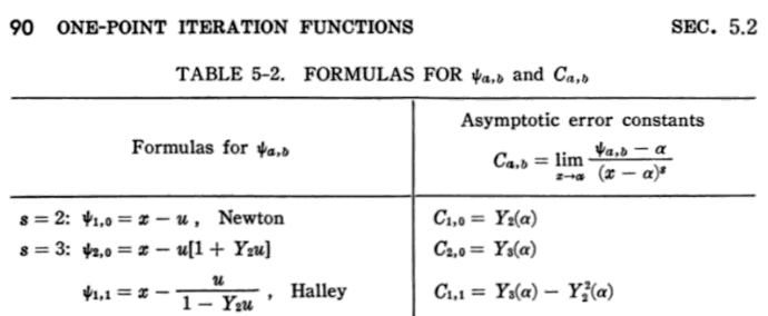
It turns out that it is not so difficult to extend the monotone convergence proof to the Euler-Chebyshev method on the logarithm of normalized price. This is however not numerically robust enough when the normalized call option price (c) is close to 1: c is between 0 and 1, and when close to 1, the misbehaves numerically due to the limited floating point accuracy. It is not a convergence issue, but a true floating point arithmetic issue. A remedy is to switch to the log of the complementary normalized price (1-c). But then the Euler-Chebyshev method is not monotone on it. Fortunately, it turns out that Halley’s method is monotone on the logarithm of the complementary normalized price. Overall, when combined, the methods lead to a much faster pricing: 3 iterations are enough to reach machine epsilon level of accuracy.
Newton, Euler-Chebyshev and Halley's methods from Iterative Methods for the Solution of Equations by Traub (1964).
For a truly robust solver, this is not enough. There are more floating point or practical convergence issues: a Bachelier based refinement for tiny prices is necessary, and polishing via the very accurate Jäckel Black-Scholes price function allows to reach closer to machine epsilon accuracy. This last polishing step end up relatively expensive compared to the rest (20% of computational time).
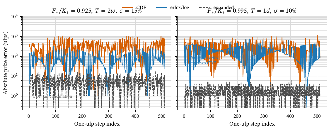
Above, I have described the journey behind creating this new solver. The reverse journey also tells an interesting tale. We could start from the Black-Scholes option price, and notice that a really accurate Black-Scholes formula implementation (close to machine epsilon) is not trivial. The textbook formula based on the normal CDF, often used in various software systems used at banks or hedge funds, is not very accurate in many cases. One should really use Peter Jäckel’s implementation everywhere, otherwise it is pointless to attempt to solve with such a high accuracy (in the paper, I thus make the Jäckel polishing step optional).
Error in the Black-Scholes price with different formulas: textbook CDF, more advanced erfcx, and Jäckel's expansion. On those realistic examples, we hit Jäckel's expansion zone.
I named the resulting solver with the somewhat cryptic name Thiophene, as Thiophene is a chemical compound with formula \[ C_4 - H_4 - S \], and C-H-S are the initials of Choi, Huh and Su.
Several years ago, I had explored accuracy and performance of different ways to imply the Black-Scholes volatility. Jherek Healy proposed some improvements over my naive algorithm on his blog. Recently, a Linkedin post mentioned a new paper from Wolfgang Schadner which presents an almost explicit formula for the implied volatility. Almost because it actually relies on some implementation of the quantile function for the inverse Gaussian distribution: it requires a specialized numerical algorithm in practice, such as the one from Giner and Smyth.
The idea is actually not new, the same formula has been used back in 2016 by Jaehyuk Choi in his github repository.
If we have a good inverse Gaussian distribution function, the algorithm is clean and simple:
using Distributions
export impliedVolatilityIG
const N = Normal()
function impliedVolatilityIG(isCall::Bool, price::T, forward, strike, timeToExpiry, df) where {T}
c, ex = normalizePrice(isCall, price, forward, strike, df)
if c >=1/ ex || c >=1 throw(DomainError(c, string("price higher than intrinsic value ", 1/ ex)))
elseif c <=0 throw(DomainError(c, "price is negative"))
end x = log(ex)
returnif abs(x) <4* eps(T)
2* quantile(N, (c +1) /2) / sqrt(timeToExpiry)
else mu =2/ abs(x)
u = cquantile(InverseGaussian(mu), c)
2/ sqrt(u * timeToExpiry)
endend
function normalizePrice(isCall::Bool, price, f, strike, df)
c = price / (f * df)
ex = f / strike
if!isCall
if ex <=1 c = c +1-1/ ex # put call parityelse#duality + put call parity c = ex * c
ex =1/ ex
endelseif ex >1# use c(-x0, v) c = (f * (c -1) + strike) / strike # in out duality, c = ex*c + 1 - ex ex =1/ ex
endendreturn c, ex
end
I was wondering how accurate it was especially for very out-of-the-money options, and how fast it was in practice. Below I compare various implementations in Julia:
Peter Jaeckel, which is arguably the industry standard.
Jherek Healy, which consists in (log-)Householder iterations on top of a good explcit initial guess.
The inverse Gaussian approach using Julia’s Distribution.jl package (as in the above code).
The inverse Gaussian approach using a basic port of statsmod R algorithm, adapted to compute the complementary quantile function. This corresponds to a different implementation of cquantile(InverseGaussian(mu),c).
I consider call optiun prices for a fixed strike K = 200 for a forward F = 100, and a time to maturity T = 1.0 year, varying the volatility from 0.02 to 4.0 in steps of 0.01. This constitute 399 samples.
Algorithm
vol RMSD
vol MAXAD
Price MAXAD
Rel. Price MAXAD
Time
Jaeckel
8.66e-16
4.00e-15
4.26e-14
1.81e-12
104 μs
Healy
1.57e-15
9.77e-15
8.53e-14
3.02e-10
107 μs
IG Distribution
7.37e-16
5.41e-15
2.84e-14
8.99e-11
246 μs
IG statsmod
7.77e-16
7.55e-15
8.24e-13
3.03e-10
311 μs
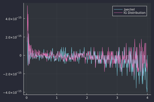
The inverse Gaussian approach is competitive but still twice slower than Peter Jaeckel’s algorithm on this example. How does the error in volatility actually look like?
Error in impled volatility of the various algorithms
The accuracy of the inverse Gaussian looks as good as Jackel’s algorithm, when using Julia’s package Distibutions.jl (it is slightly less accurate towards low vol, but slightly more accurate for high vols).
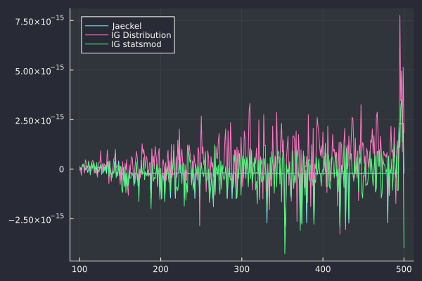
It is revealing to also look at the case of varying strikes for a fixed volatility. We consider a volatility fixed to 0.1 (or 10%) and vary the strike from 100 to 500 by steps of 1.
Algorithm
vol RMSD
vol MAXAD
Price MAXAD
Rel. Price MAXAD
Time
JAECKEL
6.50e-16
2.73e-15
7.11e-15
6.59e-12
154 μs
HEALY
6.56e-16
2.73e-15
3.55e-14
6.59e-12
110 μs
IG Distribution
1.21e-15
7.76e-15
1.78e-14
1.95e-11
1704 μs
IG statsmod
8.68e-16
4.27e-15
1.06e-14
1.32e-11
288 μs
On this example the Julia Distributions.jl leads to a performance degradation by a factor of 10 and is less accurate. It would be worth investigating exactly where lies the bottleneck, as statsmod custom implementation keeps a good performance profile.
Error in impled volatility of the various algorithms
Because it originates from the CG community, I had assumed that this was faster than the more classic scrambling ACM Algorithm 823 by Hickernell and Hong. I was wrong. It may be faster for specific use cases, but in general it is (much) slower, especially for the kind of (quasi) Monte-Carlo simulation that we use in quantitative finance.
The slowness is because we can’t just generate the next number from the sequence, we must jump to each number instead. The shuffling is implemented by jumping to some hash based location. And jumping is somewhat significantly slower than getting the next number. Furthermore, the grey code optimization can not be applied anymore.
In my code, for arbirary dimension (on the example to integrate successively a function from dimension 1 to dimension 5000 using a 100 steps on the dimension side), the Burley implementation (actually optimized to skip faster a la Quantlib instead of the original code from Burley) is 3 times slower than Algorithm 823.
It is also not obviously better on the example of Ilya M. Sobol’, Danil Asotsky in Construction and Comparison
of High-Dimensional Sobol’ Generators (Equation 6.1 and Figures 8 and 9), also reproduced by Peter Caspers.
$$
I_1 = \int_{[0,1]^d} \prod_{i=1}^d \left( 1 + 0.01(x_i - 0.5) \right) dx_1 dx_2 \dots dx_d .
$$
Absolute error in integral I1 computed with different Sobol sequences
In the Figure above, I did not use 30031 points of the sequence as in the original test, but the closest power of 2, that is 32768, which is supposed to be more optimal (the choice of 30031 is strange but actually does not really change the outcome). Except for Sobol-Harase, all use Joe Kuo new-joe-kuo-6.21201 direction numbers. Sobol-Harase uses Shin Harase niederreiter-nut-s21201.txt, which interestingly, does not fare as well as the more classic Joe Kuo set.
The results vary quite a bit depending on the random number generator used, or its seed. In the above, the Well1024a generator with default seed for the seeds of Burley’s algorithm has the lowest maximum error, but if we change the seed to 123456, this is not true anymore. Algorithm 823 (Owen and Owen-Faure-Tezuka) is not worse, and its results are also dependent on the seed (although I am under the impression that the impact is not as large). This is something that was not shown in Peter Caspers Blog.
I struggled a bit having Jack Audio Connection Kit working in Opensuse Tumbleweed.
My error was to install the jack package. The solution is actually extremely simple: use pipewire-jack instead of jack.
The state of the art of Sobol scrambling has changed slightly recently, thanks to the paper from Brent Burley of Walt Disney Studios Practical Hash-based Owen Scrambling.
Before that, ACM Algorithm 823 by Hickernell and Hong was the usual reference. Brent Burley’s algorithm is supposedly both faster and with better properties. In particular, it performs both shuffling and scrambling.
Peter Caspers implemented the new algorithm in Quantlib. It’s neat to have some decent implementation in CPP. In applying the algorithm of the paper, a few sub-optimal choices were made:
The base RNG for seeds (for the shuffling and scrambling) is Mersenne-Twister. Contrary to what I thought at the beginning, it is not used for skipping/jumping as the seeds are only set in the initialization, and are then constant for all numbers in the sequence. The skipping/jumping logic is however absent from the Quantlib CPP code, which is a bit unfortunate, but is almost trivial to code (just update the nextSequenceCounter_ variable).
There is a 4-by-4 seeding logic which looks odd. The paper code processes 4 dimensions as it is specialized to CG, although even then, it processes those 4 dimensions slightly differently: a much simpler hash function is used (it is given in the code URL inside the paper) and the seed value is not updated by the hash function: the seed is merely hashed with the dimension number, for 4 dimensions.
I don’t really see what there is to gain to follow this 4-by-4 seeding. It would be simpler and less concerning to simply use the RNG to produce N seeds where N is the number of dimensions (instead of N/4). The only possible gain with the 4-by-4 seeding is some memory (as only N/4 seeds are kept in memory), but the total amount is not significant: for 21000 dimensions, keeping all in memory takes around 656 KB (yes, 640 KB is not all we need!). The cost of 4-by-4 seeding is a potentially less random scrambling.
On the same subject, there is another new low discrepancy sequence which appears to have some good properties as well as being as fast to generate as Sobol, it’s called SZ Sequence.