Recently, I have spent some time on simple neural networks. The idea is to employ them as universal function approximators for some problems appearing in quantitative finance. There are some great papers on it such as the one from Liu et al. (2019) or Horvath et al. (2019) Deep Learning Volatility or Rosenbaum & Zhang (2021).
Incidentally, I met Liu back when I was finishing my PhD in TU Delft around 2020.
I thought I would try out what Julia offers in terms of library for neural networks. Being a very trendy subject, and Julia a modern language for the scientific community, I had imagined the libraris to be of good quality (like the many I have been using in the past). Surprisingly, I was wrong.
First, I tried SimpleChain, which just crashed (core dumped!) on a very simple example. I did not bother finding the root cause, I decided to look for another library. I then tried LUX. The execution kept going forever without returning with the @compile keyword. I probably was not being lucky, even though my code was only 10s of lines long. So I decided to use Flux, which actually is as simple to use as Pytorch, a well-known library in the Python world.
Things works with Flux, and I do manage to do many experiments. But the performance is not great. This was another surprise: Pytorch was actually faster for many tasks on the CPU (no GPU). For example, to train a multi-layer-perceptron with 4 hidden layers of 200 neurons, Julia was taking several hours, until I hit CTRL+C and launched the same training in Pytorch (which took 15 minutes). I think it may be something with AdamW optimizer and relatively wide (but not really compared to LMM stuff) networks.
Overall, the experience is pretty disappointing. Maybe it shows how much effort has been put in the Python ecosystem.
The optimization is on the x’s instead of the y’s, meaning the strike axis is fixed.
An original approach to avoid spurious modes, although I would have liked more details on it, with concrete examples of the penalty. Penalties are often challenging to get right.
A nice analysis of the asymptotic behavior in the wings, showing that an exponentially quadratic form for extrapolation corresponds to linear slopes in implied variance.
I had also explored a fixed strike axis initially (even back in 2014 - I uploaded some old notes on SSRN around this). I found it to be somewhat unstable back then, but it may well be that I did not put enough efforts into it, especially since optimizing the y’s instead of the x’s allowed for a straightforward use of B-splines, which is very attractive. It is very direct to impose monotonicity with B-splines.
The main advantage of optimizing on the x’s instead of the y’s is that the knots are defined in the more usual strike space.
Now I find interesting that someone else stumbled upon essentially the same idea starting from another point of view. There may be more merits to this parameterization than I thought.
The challenges I found with stochastic collocations were:
spurious spike when the collocation function derivative is close to zero which happens on occasion. This is not really like an extra mode - it is not smooth. Penalty or minimal slope are possible workarounds, but challenging to make robust.
dependency on the choice of knots, especially if nearly exact interpolation is required.
more minor, non-predictable runtime: the non-linear optimization is sometimes very fast, sometimes much slower. This is the case of most arbitrage-free interpolation techniques.
Leif Andersen and Mark Lake recently proposed the use of Non-Uniform Fast Fourier Transform for option pricing via the characteristic function. Fourier techniques are most commonly used for pricing vanilla options under the Heston model, in order to calibrate the model. They can be applied to other models, typically with known characteristic function, but also with numerically solved characteristic function as in the rough Heston model, and to different kind of payoffs, for example variance/volatility swaps, options. The subject has been vastly explored already so what’s new with this paper?
At first, it was not obvious to me. The paper presents 3 different approaches, two where the probability density and cumulative density is first computed at a (not so sparse) set of knots and the payoff is integrated over it. The remaining approach is the classic one presented in the Carr and Madan paper from 1999 as well as in most of the litterature on the subject. The only additional trick is really the use of NUFFT along with some clever adaptive quadrature to compute the integral.
I thought the main cost in the standard Fourier techniques was the evaluation of the characteristic function at many points, because the characteristic function is usually relatively complicated. And, in practice, it mainly is. So what does the new NUFFT algorithm bring? Surely the characteristic function must still be evaluated at the same points.
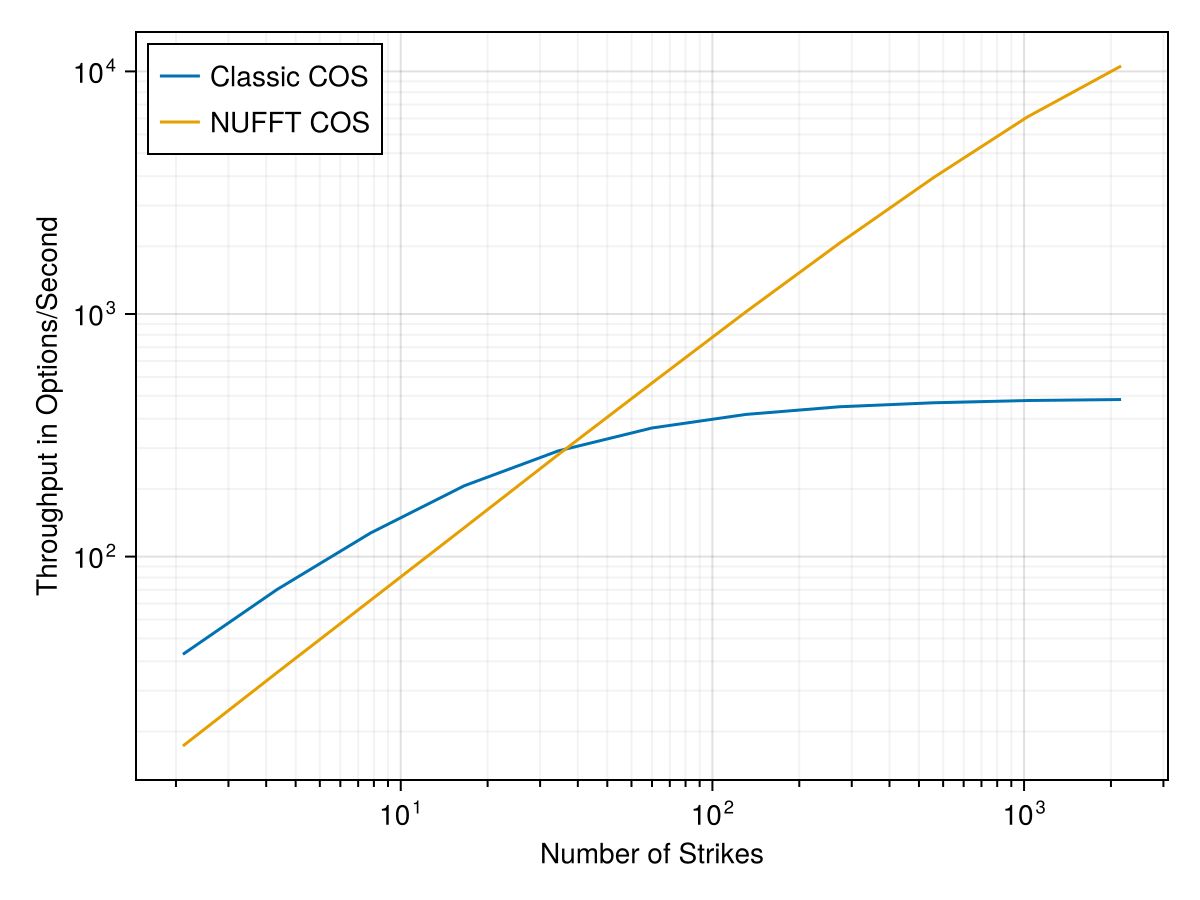
The NUFFT becomes interesting to compute the option price at many many strikes at the same time. The strikes do not need to be equidistant and can be (almost) arbitrarily chosen. In Andersen and Lake paper, even a very fast technique such as the COS method reaches a threshold of option per second throughput, as the number of strikes is increased, mainly because of the repeated evaluation of the sum over different strikes, so the cost becomes proportional to the number of strikes.
Evaluating at many many points becomes not much more expensive than evaluating at a few points only. This is what opens up the possibilities for the first 2 approaches based on the density.
It turns out that it is not very difficult to rewrite the COS method so that it can make use of the NUFFT as well. I explain how to do it here. Below is the throughput using NFFT.jl Julia package:
Throughput on the Heston model with M=256 points.
While a neat trick, it is however not 100% clear to me at this point where this is really useful: calibration typically involve a small number of strikes per maturity.
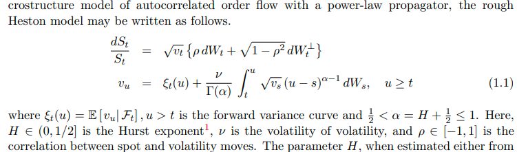
According to the litterature, the initial forward variance curve is typically built from the implied volatilities through the variance swap replication: for each maturity, the price of a newly issued variance swap is computed to this maturity, using the implied volatilities for this maturity. Then we may compute the forward variance by interpolating linearly the variance swap prices and differentiating. This leads to the plot below.
Forward variance curves for SPX500 as of October 2024.
One immediate question is how much does the truncation range play a role in this forward variance curve? Above, we plot the replications prices based on filtering the input data up to 10 Delta / 90 Delta for each maturity. Beyond this range, liquidity is usually much lower and the reliability of the input quotes may not be as good. The short end, and not so short forward variance up to 4 years is quite different. The long end is more aligned with something that looks like a basis spread between the two curves.
We may also calibrate the forward variance curve model directly to the implied volatilities during the model calibration, at the same time as the other stochastic volatility parameters (using a time-dependent correlation and vol-of-vol). This time-dependent Heston parameterization has effectively 3 parameters per expiry. In this case, we may want to also filter the input data to focus on the 10 Delta / 90 Delta range as we expect the stochastic volatility model to fit well where it matters the most - where the vanillas are liquid.
In the figure above, we also plot the forward variance curve implied by the model, through a calibration against vanilla options. We can see it is again quite different.
If we were to use the true replication based forward variance curve, we would effectively attempt to fit far away vols in the wings, which somehow seems wrong. Now if the model was able to fit everything well there would be no issue, but with 3 parameters per maturity, a choice has to be made. And the choice of the full replication does not look particularly great, as we fit exactly something that is not liquid.
I recently saw a news about a great new simulation scheme for the Heston model by Abi Jaber.
The paper suggests it is better than the popular alternatives such as the QE scheme of Leif Andersen. Reading it quickly, perhaps too quickly, I had the impression it would be more accurate especially when the number of time-steps is small.
The scheme is simple to implement so I decided to spend a few minutes to try it out. I had some test example for the DVSS2X scheme pricing a vanilla at-the-money option with Heston parameters v0=0.04, kappa=0.5, theta=0.04, rho=-0.9, sigma=1.0, and a time to maturity of 10 years. I don’t remember exactly where those parameters come from, possibly from Andersen paper. My example was using 8 time-steps per year, which is not that much. And here are the results with 1M paths (using scrambled Sobol):
N
Scheme
Price
Error
1M
DVSS2X
13.0679
-0.0167
IVI
13.0302
-0.0545
4M
DVSS2X
13.0645
-0.0202
IVI
13.0416
-0.0431
With Sobol scrambling and 1 million paths, the standard error of the Monte-Carlo simulation is lower than 0.01 and the error with this new IVI scheme is (much) larger than 3 standard deviations, indicating that the dominating error in the simulation is due to the discretization.
It is not only less accurate, but also slower, because it requires 3 random numbers per time-step, compared to 2 random numbers for QE or DVSS2X. The paper is very well written, and this small example may not be representative but it does cast some doubts about how great is this new scheme in practice.
While writing this, I noticed that the paper actually uses this same example, it corresponds to their Case 3 and it is indeed not obvious from the plots in the paper that this new IVI scheme is significanly better. There is one case, deep in the money (strike=60%), and very few time-steps (2 per year for example):
N
Steps/Year
Scheme
Price
Error
4M
2
DVSS2X
44.1579
-0.1721
IVI
44.2852
-0.0449
4
DVSS2X
44.2946
-0.0353
IVI
44.3113
-0.0187
8
DVSS2X
44.3275
-0.0025
IVI
44.3239
-0.0061
So the new scheme works reasonably well for (very) large time-steps, better than DVSS2 and likely better than QE (although, again, it is around 1.5x more costly). For smaller steps (but not that small), it may not be as accurate as QE and DVSS2. This is why QE was such a big deal at the time, it was significantly more accurate than a Euler discretization and allowed to use much less time-steps: from 100 or more to 10 (a factor larger than 10). IVI may be an improvement for very large step sizes, but it will matter much less for typical exotics pricing where observation dates are at worst yearly.
Update June 19, 2025
Out of curiosity I wondered how it behaved on my forward start option test. In the Table below I use 4M paths.
Scheme
Steps/Year
Price
DVSS2X
4+1
0.0184
80
0.0196
QE
4+1
0.0190
160
0.0196
IVI
4+1
0.0116
80
0.0185
160
0.0191
Clearly, the IVI scheme is not adequate here, it seems to converge very slowly. The price with 4+1 steps is very off, especially compared to the other schemes. The implementation is fairly straighforward, so the IVI scheme may well have a flaw.
Fabrice Rouah wrote two books on the Heston model: one with C# and Matlab code, and one with VBA code. The two books are very similar. They are good in that they tackle most of the important points with the Heston model, from calibration to simulation. The calibration part (chapter 6) is a bit too short, it would have been great if it presented the actual difficulties with calibration in practice and went more in-depth with the techniques.
There is a full chapter on the time-dependent Heston model and it presents there the expansion of Benhamou, Gobet and Miri. The code is relatively annoying to write, so it’s great to have code available for it in the book. It is not so common for books to give source code with it, if you read the free access pages on Wiley’s website, you can download the source code.
Also the methodology used is the correct one to follow: first, reproduce the numbers of the original paper, second, use the approximation in a concrete calibration. There are however two major problems:
The code has errors.
The expansion is not really good in practice.
There are two errors in the code: one in the cross derivative of PHIgxy2 (first order on x and second order on y), and one in the second order cross derivative of the Black-Scholes price dPdx2dy2.
The formula for the piecewise-constant coefficients also contains errors: for example, the total variance variable wT is wrong. It should be a double sum instead of the standard constant Heston like formula. Finally, the many sums are rederived in the book, differently from the paper and are not simplified (unlike in the paper where they are all single sums).
Indeed, with the original code from Rouah, the prices in the table of the paper from Benhamou Gobet and Miri are not reproduced to the last digit. With the above changes, they are.
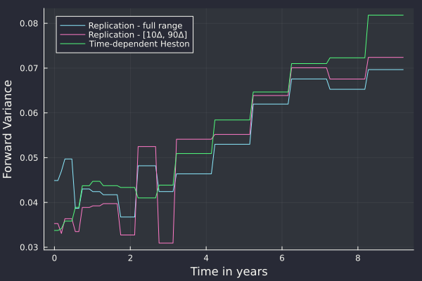
On the second point, it is surprising that the book does not mention that the approximation is not great. In particular, it does not mention that the calibrated parameters between Table 9.6 and Table 9.3 are vastly different (except for v0). The calibrated smile is plotted, which is great, but it is only plotted with the approximation formula. Plotting the same using the nearly exact semi-analytical representation of vanlla option prices would have been enlightening. We do it below, as Fabrice Rouah gives all the inputs (a very good thing):
DJIA 37 days maturity.
DJIA 226 days maturity.
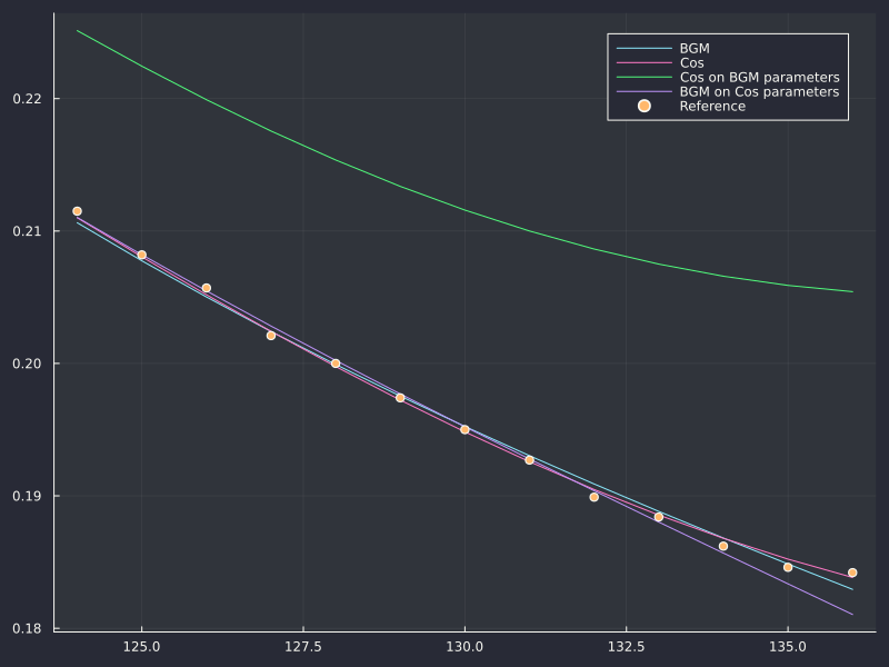
It looks like in the range the calibration stays in the range of applicability of the formula, which is good, but not necessarily always true. The main issue is however that the calibrated parameters with the approximation are not necessarily a good guess for the parameters of the true time-dependent Heston model, precisely because the actual optimal parameters are way outside the range where the approximation is accurate. This is clear in the 226D plot, the best fit from the approx (which is great) ends up a not so good fit for the real time-dependent Heston model. Somewhat interestingly, the approx is actually not so bad on the actual optimal parameters, gotten from a calibration of the model with the Cos method - it is however a less good fit with the approx than the optimal parameters gotten from a calibration of the model with the approximation.
More recently, Pat Hagan proposed a new approximation for the model, based on a SABR mapping. It seems a bit more precise than the approximation of Benhamou Gobet and Miri, but is not great either. And it is disappointing that the paper does not present any number, nor any plot to assess the quality of the approximation given. Van der Zwaard gives some relatively realistic yet simple set of parameters for the Heston model (using Hagan’s reparameterization with constant expected variance = 1) and on those, the approximated prices of at-the-money options are just not usable:
If we consider his Table 5.9 (maturity = 1.75 year), we have the following
Method
Price
Error
BGM
4.2206
0.21
Hagan
3.3441
0.66
Reference
4.0039
0
With Table 5.10 (maturity = 1.3 year), it is even worse:
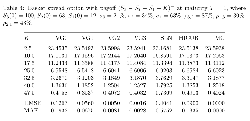
More recently, I applied the idea to approximate arithmetic Asian options prices by using the geometric Asian option price as a proxy (with some adjustments). This worked surprisingly well, and is competitive with the best implementations of Curran approach to Asian options pricing. I quickly noticed that I could apply the same idea to approximate Basket option prices, and from it obtain another approximation for vanilla options with cash dividends through the mapping described by J. Healy. Interestingly the resulting approximation is the most accurate amongst all other approximations for cash dividends.
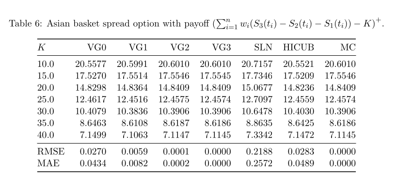
During my Easter holidays, I took the time to further extend the idea to cover general spread options such as Asian Basket spread options. I was slightly surprised at the resulting accuracy: the approximation is by far more accurate than any other published approximation on this problem.
Somewhat interestingly, I noticed that the first order expansion (which is not much more accurate than the proxy itself) seemed to correspond to a previously published approximation from Tommaso Pellegrino, an extension of Bjerksund-Stensland approximation for spread options, although my derivation is very different and allows for higher-order formulae.
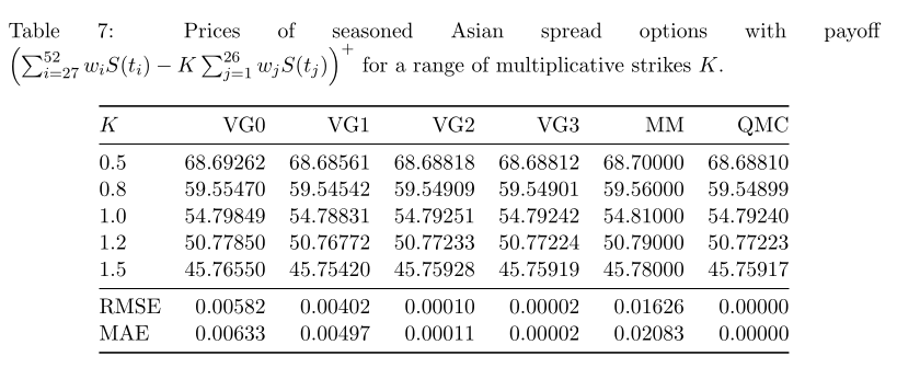
Below is an excerpt of some of the results
Original example from Deelstra et al. for an Basket spread option.
Original example from Deelstra et al. for an Asian Basket spread option. The Taylor approximation perform even better due to the Asianing.
Original example from Martin Krekel for an Asian spread option. It was actually challenging to compute accurate Quasi Monte-Carlo prices.
The MM of Martin Krekel consists in a one-dimensional integration of two lognormal moment-mached distributions. It seems that the one-dimensional integration (which is exact for simple spread options) does not really improve the accuracy for the more general asian spread option case: the loss of accuracy due to moment matching dominates the error.
My 12 years old child recently had a presentation to do with 3 other children for school, the subject was food and health.
It was particularly difficult to organize the children and one of the children came with a full presentation with text, generated by an LLM (possibly corrected by the parents).
At first, I thought this was just cheating and completly useless. Furthermore, he failed to read properly the details of the subject, and much of it wasn’t relevant.
Then they did a second round together, at another parents home. And the outcome was even worse, in that it was even further away from the subject and had equally strong use of LLM.
I decided to try out some LLM queries on this subject (in French) after I installed a few local LLMs via Ollama. Ollama makes it really easy to run an LLM locally. The drawback is that
the models have not necessarily been trained very recently, for example Llama 3.2 was trained in 2021 according to itself. I tried Llama 3.2 and Mistral, with respectively 3B and 7B parameters. This is another
drawback, it is challenging to run much larger models as they would require too much RAM. Ollama github page mentions 32 GB to run the 33B models.
The answers we get are not bad, but they are not great either. For example to the question
En quoi les besoins alimentaires dépendent de l’age, du sexe et de l’activité physique de chaque individu?
Les besoins alimentaires de chaque individu peuvent être influencés par différents facteurs tels que son âge, son genre, sa taille, son poids, son niveau
d’activité physique et son état de santé.
Par exemple, les enfants ont besoin de plus de calories et de nutriments pour leur croissance rapide. De même, les femmes enceintes et allaitantes ont des
besoins alimentaires différents car elles devront fournir les éléments nécessaires à la formation du fœtus ou au lait maternel.
Les hommes et les femmes ont également des besoins alimentaires différents en raison de leurs besoins nutritionnels uniques, tels que la besoin plus élevé
de protéines chez les hommes en raison de leur plus grand poids moyen. En outre, certains nutriments sont spécifiquement importants pour des groupes
spécifiques d’individus, par exemple, les femmes en âge de procréer ont besoin d’un apport plus élevé en fer et folate pour s’assurer que leur fœtus ait un
développement normal.
Enfin, les individus qui sont plus actifs physiquement ou ceux qui ont une activité physique professionnelle exigeante ont des besoins alimentaires
différents car ils nécessitent plus d’énergie pour maintenir leur niveau d’activité. Ils doivent consommer davantage de calories et de nutriments pour
répondre à leurs besoins énergétiques supérieurs, ce qui peut inclure des aliments riches en protéines, vitamines et minéraux.
En bref, les besoins alimentaires de chaque individu peuvent être influencés par différents facteurs tels que son âge, son genre, sa taille, son poids, son
niveau d’activité physique et son état de santé. Il est donc important de comprendre ces facteurs pour assurer que nous consommons une alimentation adaptée à
nos besoins nutritifs uniques.
The introduction and the conclusion are the same. Closely repeated words are another issue: spécifiquement. Furthermore, this word is likely a bad translation from English in the sentence.
“spécifiquement importants” does not sound quite correct in French. Finally, it’s funny that they always produce the same structure of answer, small intro, a few points, and “En bref…”. At first it looks good, but very quickly, you
understand it as noise. In fact if we analyze the points given as answer by LLMs, we start to notice that they are not as distinct as their presentation and wording suggest. It is not uncommon to see very similar sentences in distincts enumerated points.
Google’s internal LLM is not great either as it does not necessarily give the correct context for understanding.
It makes you believe that 1g of protein has 4 calories. But which kind of calorie? the large Calorie (kcal or C) or the small calorie (c) ? The reality is 4000 c or 4 kcal. Btw, I did not know both were introduced by French scientists, and that the large calorie variant was from Marcelin Berthelot. This is a neat feature of websites or books compared to LLMs, you get more contextual information.
The main problem is that the LLMs tend to bring those lists on you, splitting into categories it decided itself, which are most of the time, not categories most human beings would choose.
Here it is to the point that children forget about the actual detailed guidelines given to them, because any of those LLM answers look so convincing. This leaves me with the impression that if they had had no LLM, no internet, no computer, they would have produced a better output.
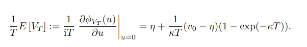
An interesting idea to calibrate the Heston model in a more stable manner and reduce the calibration time is to make use of variance swap prices. Indeed, there is a simple formula for the theoretical price of a variance swap in the Heston model.
It is not perfect since it approximates the variance swap price by the expectation of the integrated variance process over time. In particular it does not take into account eventual jumps (obviously), finiteness of replication, and discreteness of observations. But it may be good enough. Thanks to this formula, we can calibrate three parameters of the Heston model: the initial variance, the long-term mean variance, and the speed of mean reversion to the term-structure of variance swaps. We do not need market prices of variance swaps, we may simply use a replication based on market vanilla options prices, such as the model-free replication of Fukasawa.
The idea was studied in the paper Heston model: the variance swap calibration by F. Guillaume and W. Schoutens back in 2014. The authors however only used the variance swap calibration as an initial guess. How bad would it be to fix the parameters altogether, as in a variance curve approach?
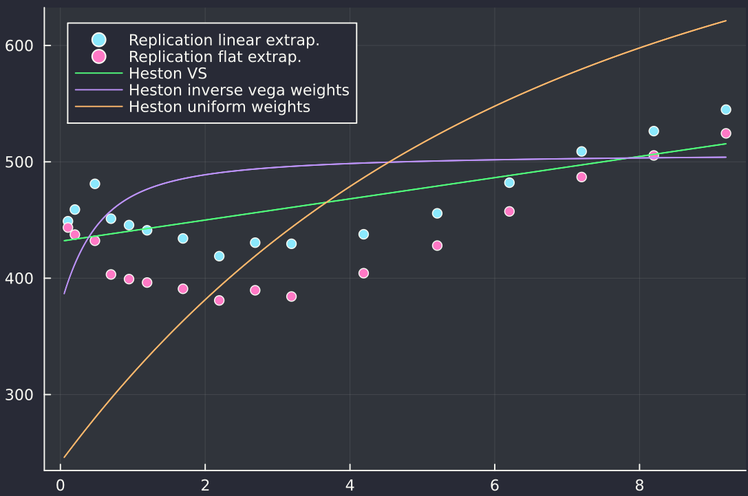
It turns out it can be quite bad since the Heston model does not allow to represent many shapes of the variance swap term structure. Below is an example of term-structure calibration on SPX as of October 2024.
Term-structure of variance swap prices.
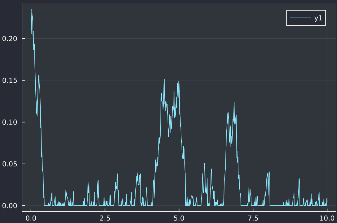
The term-structure is V-shaped, and Heston can not fit well to this. The best fit leads to non-sensical parameters with a nearly zero kappa (mean reversion speed) and an exploding long-term mean theta. The next figure shows why it is non-sensical: because the kappa is very small, the variance will very often reach zero.
Sample path of the variance process (in terms of vol) using the Euler scheme with full truncation.
The calibration using inverse vega weights on vanilla option prices leads a not much worse fit of the variance swap term structure, but exhibits a much to high, unrealistic vol-of-vol of 184%, while a calibration on equally weighted option prices does not fit the term structure well at all.
Somewhat interestingly, the Double-Heston model allows to fit the term-structure much better, but it is far from obvious that the resulting calibrated parameters are much more realistic as it typically leads to process with very small kappa or a process with very small theta (but as there are two processes, it may be more acceptable).
Previously, I had explored a similar subject for the Schobel-Zhu model. It turns out that Heston is not much more practical either.
I recently upgraded a desktop computer, and to my surprise, the new motherboard was not fully supported by most Linux distributions.
The main culprit was the network adapter, although the secure boot setup gave me lots of troubles as well. I had only a small usb key (2GB)
and most (all?) live distributions do not fit on 2GB anymore. With the exception of Ubuntu images, I did not manage to boot from USB hard drive where I dumped the live image ISO, due to Secure boot
related issues, even when disabling the feature or changing the settings in the BIOS. Using the small USB key worked with Secure boot enabled only.
So I had to find a distribution with a small size and with a new kernel which supported the network adapter (6.13+). I tried the rawhide Fedora, which has a small network install image, but that just did not work, because it’s too alpha.
I thought most rolling distributions would fit the bill. It turns out they don’t, EndeavourOS or Manjaro have relatively recent live install but (a) they are not small enough to fit on the USB key and (b) the images are a few months old where the kernel is too old.
OpenSuse Tumbleweed provides a daily updated network installer iso (and a live CD), this is the only thing that worked, and it worked well.
Overall I was a bit surprised that it was so challenging to find an installable distribution with the latest kernel.