Measuring Roughness with Julia
I received a few e-mails asking me for the code I used to measure roughness in my preprint on the roughness of the implied volatility. Unfortunately, the code I wrote for this paper is not in a good state, it’s all in one long file line by line, not necessarily in order of execution, with comments that are only meaningful to myself.
In this post I will present the code relevant to measuring the oxford man institute roughness with Julia. I won’t go into generating Heston or rough volatility model implied volatilities, and focus only on the measure on roughness based on some CSV like input. I downloaded the oxfordmanrealizedvolatilityindices.csv from the Oxford Man Institute website (unfortunately now discontinued, data bought by Refinitiv but still available in some github repos) to my home directory
using DataFrames, CSV, Statistics, Plots, StatsPlots, Dates, TimeZones
df = DataFrame(CSV.File("/home/fabien/Downloads/oxfordmanrealizedvolatilityindices.csv"))
df1 = df[df.Symbol .== ".SPX",:]
dsize = trunc(Int,length(df1.close_time)/1.0)
tm = [abs((Date(ZonedDateTime(String(d),"y-m-d H:M:S+z"))-Date(ZonedDateTime(String(dfv.Column1[1]),"y-m-d H:M:S+z"))).value) for d in dfv.Column1[:]];
ivm = dfv.rv5[:]
using Roots, Statistics
function wStatA(ts, vs, K0,L,step,p)
bvs = vs # big.(vs)
bts = ts # big.(ts)
value = sum( abs(log(bvs[k+K0])-log(bvs[k]))^p / sum(abs(log(bvs[l+step])-log(bvs[l]))^p for l in k:step:k+K0-step) * abs((bts[k+K0]-bts[k])) for k=1:K0:L-K0+1)
return value
end
function meanRoughness(tm, ivm, K0, L)
cm = zeros(length(tm)-L);
for i = 1:length(cm)
local ivi = ivm[i:i+L]
local ti = tm[i:i+L]
T = abs((ti[end]-ti[1]))
try
cm[i] = 1.0 / find_zero(p -> wStatA(ti, ivi, K0, L, 1,p)-T,(1.0,100.0))
catch e
if isa(e, ArgumentError)
cm[i] = 0.0
else
throw(e)
end
end
end
meanValue = mean(filter( function(x) x > 0 end,cm))
stdValue = std(filter( function(x) x > 0 end,cm))
return meanValue, stdValue, cm
end
meanValue, stdValue, cm = meanRoughness(tm, ivm, K0,K0^2)
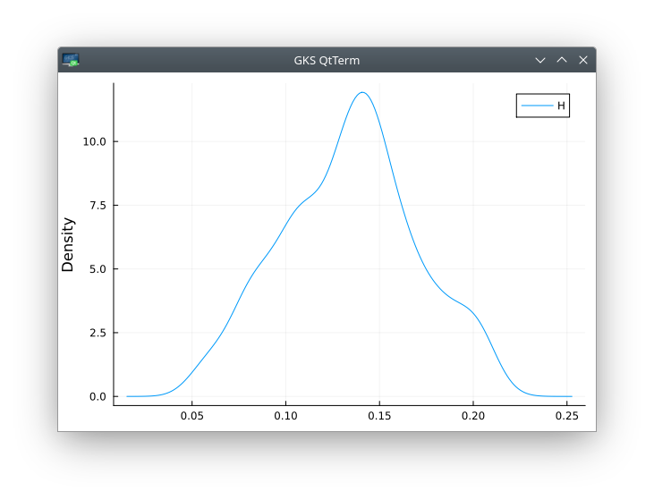
density(cm,label="H",ylabel="Density")