The Dupire equation for local volatility has been derived under the assumption of Martingality, that means no dividends or interest rates.
The extension to continuous dividend yield is described in many papers or books:
With cash dividends however, the Black-Scholes formula is not valid anymore if we suppose that the asset jumps at the dividend date of the dividend amount. There are various relatively accurate
approximations available to price an option supposing a constant (spot) volatility and jumps, for example, this one.
Labordère, in his paper Calibration of local stochastic volatility models to market smiles, describes a mapping to obtain the market local volatility corresponding to the model with jumps, from the local volatility of a pure Martingale. Assuming no interest rates and no proportional dividend, the equations looks particularly simple, it can be simplified to:
While it appears very simple, in practice, it is not so much. For example, let’s consider a single maturity smile (a smile, constant in time) as the market reference spot vols. Which volatility should be used in the formula for \( \hat{C} \)? logically, it should be the volatility corresponding to the market option price of strike K and maturity T. The numerical derivatives will therefore make use of 4 distinct volatilities for K, K+dK, K-dK and T+dT. In the pricing formula,
we can wonder if at T+dT, the price should include the eventual additional dividend or not (as it is infinitesimal, probably not).
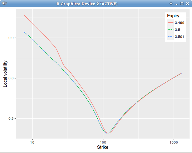
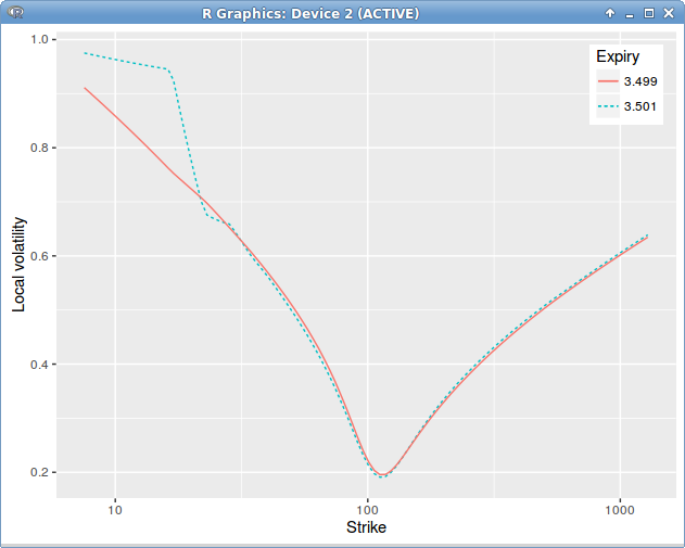
It turns out that applying the above formula leads to jumps in time in the local volatility, around the dividend date, even though our initial market vols were flat in time.
Dupire Local Volatility under the spot model with jump at dividend date = 3.5 on a single constant in time spot smile.
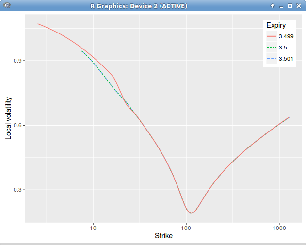
The mistake is not that clear. It turns out that, when using a single volatility slice, extrapolated in constant manner, the option continuity relationship around the dividend maturity is not respected. We must have
Dupire Local Volatility under the spot model with jump at dividend date = 3.5, introducing a slice before the dividend date to enforce the price continuity relationship.
Look, when we shift by the dividend!
The slightly funny shape of the local volatility in the left wing, before the dividend, is due to linear extrapolation use.
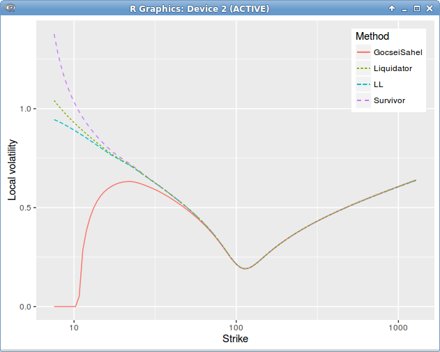
Interestingly, there is quite a difference in the local volatility for low strikes, depending on the dividend policy, here is how it looks for a single dividend with liquidator vs survivor policy.
Dupire Local Volatility under the spot model with jump at dividend date = 3.5 on a single constant in time spot smile.
The analytical approximations lead to another different local volatility from both policies, but don’t differ much from each other. Guyon and Labordere approximation based on the skew averaging technique of Piterbarg, not displayed here, is the worst. Gocsei-Sahel approximation has some issues for the lower strikes, the Etore-Gobet expansions on strike or on Lehman and the Zhang approximation are very stable and accurate, except for the very low strikes, where the dividend policy starts playing a more important role.
Those differences however don’t impact the prices very much as the prices with the various methods (excepting the Guyon-Labordère approximation) are very close, and differ of a magnitude much smaller than the error to the true price.
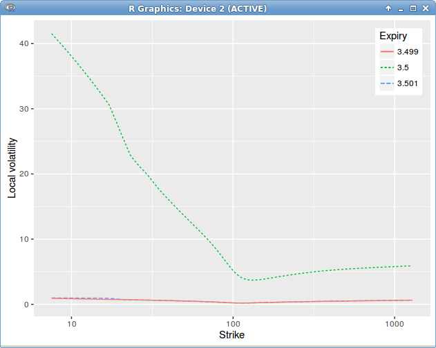
The continuous yield approach consist in first building the equivalent Black volatility and use the regular Dupire on it. This is qualitatively different from a cash dividend jump, and is closer to a proportional dividend jump. Note that there is still a jump in the continuous yield local volatility:
Dupire Local Volatility under the forward model.
The huge spike at 3.5 don’t allow us to see much about what’s happening around:
Dupire Local Volatility under the forward model.
Overall, when the dividends happens early, the Dupire formula for cash dividends works well, but when the dividends are closer to maturity there is a marked bias in the prices, that does not disappear with more steps in the FDM. Typically, at \(0.7T\), the absolute price error is around 0.01 and more or less constant accross strikes. In contrast, the classic continuous yield Dupire behaves well, despite the spike, and the error decreases with the number of steps, I obtain around 5E-4 with 500 steps.
I would have expected a much better accuracy from Labordère’s approach, it’s still not entirely clear to me if there is not an error lurking somewhere. This is how an apparently simple formula can become a nightmare to use in practice.
Update: A follow-up to this post where I resolve the mysterious remaining error.
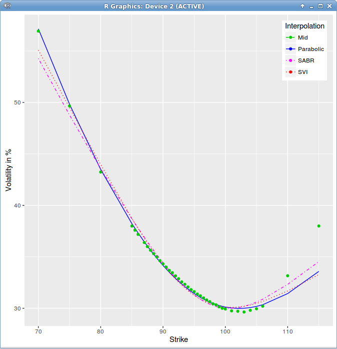
In a previous post, I took a look at least squares spline and parabola fits on AAPL 1m options market volatilities. I would have imagined SVI to fit even better since it has 5 parameters, and SABR to do reasonably well.
It turns out that the simple parabola has the lowest RMSE, and SVI is not really better than SABR on that example.
SVI, SABR, least squares parabola fitted to AAPL 1m options
Note that this is just one single example, unlikely to be representative of anything, but I thought this was interesting that in practice, a simple parabola can compare favorably to more complex models.
A while ago, I have applied a relatively simple adaptive Filon quadrature to the problem of volatility swap pricing. The Filon quadrature is an old quadrature from 1928 that allows to integrate oscillatory integrand like \(f(x)\cos(k x) \) or \(f(x)\sin(k x) \). It turns out that combined with an adaptive Simpson like method, it has many advantages over more generic adaptive quadrature methods like Gauss-Lobatto, which is often used on similar problems.
Flinn derived a similar quadrature, but taking into account the derivative values, which are likely to be easily available on those problems. This produces a even more robust quadrature and of higher convergence order.
I was curious how practical this would be on Heston or other stochastic volatility models with a known characteristic function. It turns out it produces a very competitive performance-wise and very stable option pricing method: it can be up to five times faster than an adaptive Gauss-Lobatto within a calibration. I found it faster and more robust than the Cos method (especially as it is quite tricky to guess properly the truncation of the Cos method).
If you are interested, you will find much more details in this document.
In my paper “Fast and Accurate Analytic Basis Point Volatility”,
I use a table of Chebyshev polynomials to provide an accurate representation of some function. This is
an idea I first saw in the Faddeeva package to
represent the cumulative normal distribution with high accuracy, and high performance. It is also
simple to find out the Chebyshev polynomials, and which intervals are the most appropriate for those, which
makes this technique quite appealing.
Still, it would have been nice to have also a more visually appealing rational function representation, as W. Shaw
did for the cumulative normal distribution (again). Popular algorithms to find the best rational function representation
seem to be minimax or Remez. But I could not find an open-source library where those were implemented. There is an
interesting implementation in chebfun but this depends on Matlab.
The Numerical recipe book provides a simple algorithm in chapter 5.13, not looking for the best possible rational function, but just for one
that would be “good enough”. Interestingly, the first part of the algorithm merely computes a least squares solution
on some chebyshev like nodes. I however quickly noticed funny behaviors with the code: it could produce a worse fit
for a higher order numerator or denominator. Then I tried some least squares python code which ended up being just buggy:
I am not sure what the code actually does with all the numpy and scipy magic, it gives solutions with poles in the data, and clearly not the least squares solution. I can’t fully understand why one would propose such a code.
It turns out that I had an alternative very basic least squares polynomial fit implementation, which is based on this matrix representation.
I wondered if it would be as prone to errors as Numerical recipe code (where they use SVD internally to solve).
The answer is: it depends. It depends on the solver used. If I use a QR solver, then the implementation looks robust on my test data,
much more than Numerical recipe code. If I use LU, it just fails in some cases. If I use SVD, it is sometimes better sometimes worse than Numerical recipe.
Interestingly, I thought, that, maybe, a gradient descent could allow to regain the lost accuracy with SVD, using
as starting point, the SVD guess. However, it does not work, it just converges more or less to the same (bad) solution.
Another interesting point, is that the using QR decomposition (instead of SVD)
in the Numerical recipe implementation resulted in a much better solution, better even than my basic least squares fit,
which looked robust, but was actually not so much.
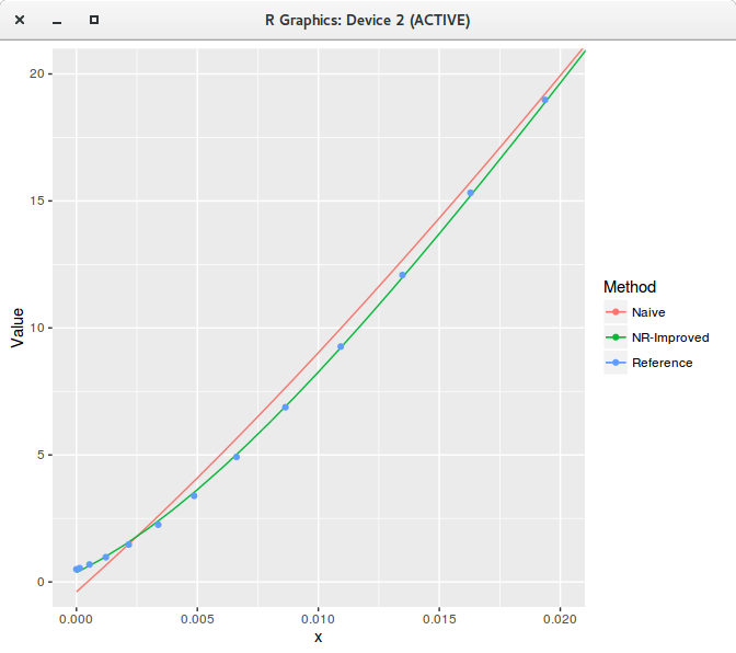
Armed with this improved Numerical recipe code (labeled NRI), here is a comparison of fit of my naive code (with QR) against the improved numerical recipe
(NRI) for a polynomial of degree 20. We can visually see the difference (when we zoom)!
Least squares polynomial fit of degree 20 zoomed.
The RMSE difference on the full interval [0,1] on 1000 equidistant points is huge:
Method
RMSE
Polynomial Naive
0.234
Polynomial NRI
0.039
Rational NRI
0.001
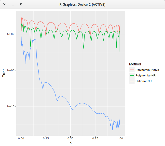
A 10/10 rational function (numerator of degree 10, denominator of degree 10) gives a much better fit than a polynomial of degree 20. It is interesting to look at the error
visually to understand how large is the difference:
Least squares polynomial fit error of degree 20.
I still can draw a conclusion to my quest for a rational function approximation: I won’t find a good one with the
change of variables I am using in my paper, as I would imagine the least squares solution to be at worst around one order of magnitudes
away from the minimax. The errors I got suggest I would need a few rational functions, maybe 3 or more, and then it does not look
all that appealing compared to the table of Chebyshev polynomials.
I thought this was a good example of how relatively simple numerical tasks can be challenging in practice.
Update - The paper now contains a solution for the normal volatility inversion problem with only 3 rational functions.
I am experimenting a bit with least squares splines. Existing algorithms (for example from the NSWC Fortran library) usually work
with B-splines, a relatively simple explanation of how it works is given in this paper (I think this is how De Boor coded it in the NSWC library).
Interestingly there is an equivalent formulation in terms of standard cubic splines, although it seems that the
pseudo code on that paper has errors.
Least squares splines give a very good fit for option implied volatilities with only a few parameters.
In theory, the number of parameters is N+2 where N is the number of interpolation points.
I tried on some of my AAPL 1 month option chain, with only 3 points (so 2 splines or 5 free parameters).
least squares spline on 1m AAPL options.
It would be interesting to add the natural constraints so that it can be linearly extrapolated. Maybe for next time.
I recently had some fun trying to work directly with the option chain from the Nasdaq website.
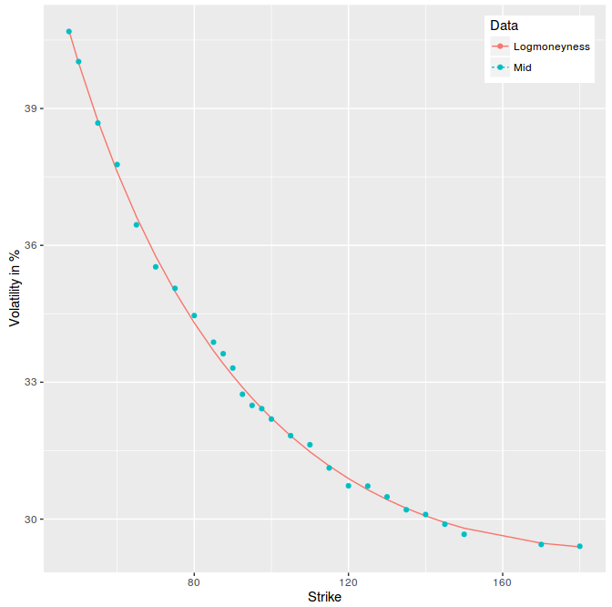
The data there is quite noisy, but a simple parabola can still give an amazing fit. I will consider the options of maturity two years as illustration.
I also relied on a simple implied volatility algorithm that can be summarized in the following steps:
Compute a rough guess for the forward price by using interest, borrow curves and by extrapolating the dividends.
Imply the forward from the European Put-Call parity relationship on the mid prices of the two strikes closes to the rough forward guess. A simple linear interpolation between the two strikes can be used to compute the forward.
Compute the Black implied volatilities as if the option were European using P. Jaeckel algorithm.
Calibrate the proportional dividend amount or the growth rate by minimizing, for example with a Levenberg-Marquardt minimizer, the difference between model and mid-option prices corresponding to the three strikes closest to the forward. The parameters in this case are effectively the dividend amount and the volatilities for Put and Call options (the same volatility is used for both options). The initial guess stems directly from the two previous steps. American option prices are computed by the finite difference method.
Solve numerically the volatilities one by one with the TOMS748 algorithm so that the model prices match the market mid out-of-the-money option prices.
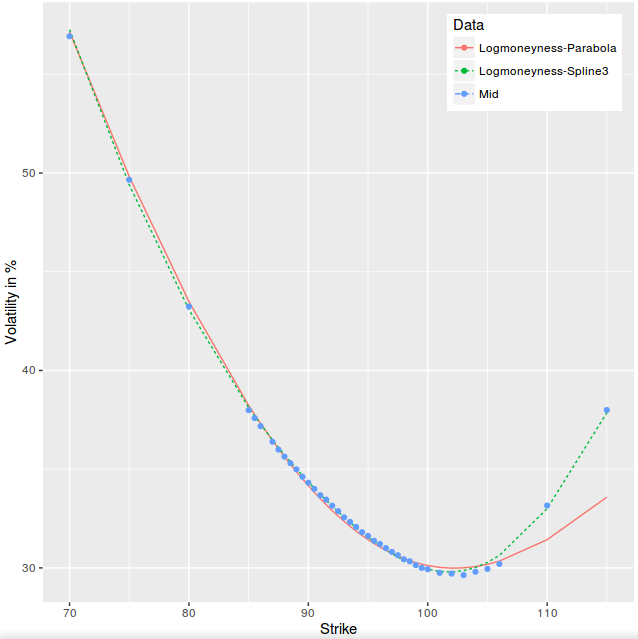
Then I just fit a least squares parabola in variance on log-moneyness, using options trading volumes as weights and obtain the following figure:
least squares parabola on 2y AAPL options.
Isn’t the fit just amazing?
Even if I found it surprising, it’s probably not so surprising. The curve has to be smooth, somewhat monotone, and will be therefore like a parabola near the money. While there is no guarantee it will fit that well far away, it’s actually a matter of scale. Short maturities will lead to not so great fit in the wings, while long maturities will correspond to a narrower range of scaled strikes and match better a parabola.
The option chain on Yahoo finance shows an implied volatility number for each call or put option in the last column.
I was wondering a bit how they computed that number. I did not exactly find out their methodology, especially since we don’t even know the daycount convention used, but
I did find that it was likely just garbage.
A red-herring is for example the large discrepancy between put vols and call vols. For example strike 670, call vol=50%, put vol=32%.
This suggests that the two are completely decoupled, and they use some wrong forward (spot price?) to obtain those numbers. If I compute
the implied volatilities using put-call parity close to the money to find out the implied forward price, I end up with ask vols of 37% and 34% or call and put mid vols of 33%.
By considering the put-call parity, I assume European option prices, which is not correct in this case. It turns out however, that with the low interest rates we live in, there is nearly zero additional value due to the American early exercise.
I am not sure what use people can have of Yahoo implied volatilities.
Tufte proposes interesting guidelines to present data, or even to design written semi-scientific papers or books. Some advices
are particularly relevant like the careful use of colors (don’t use all the colors of the rainbow just because you can), and
in general don’t add lines in a graph or designs that are not directly relevant to the message that needs to be conveyed. There is also a parallel
with Feynman message against (Nasa) Powerpoint presentations. But other inspirations, are somewhat doubtful.
He seems to have a fetish for old texts. They might be considered pretty, or interesting in some ways, but
I don’t find them particularly easy to read. They look more like esoteric books rather than practical books. If you want to write
the new Bible for your new cult, it’s probably great, not so sure it’s so great for a more simple subject.
Also somewhat surprisingly, his own website is not very well designed, it looks like a maze and very end of 90s.
I experimented a bit with the Tufte latex template. It produced that document for example. But someone rightfully pointed out to me
that the reference style was not really elegant, that it did not look like your typical nice science paper references. Furthermore,
using superscript so much could be annoying for someone used to read math and consider superscript numbers as math symbols.
In general, there seems to be a conflict between the use of Latex and many Tufte guidelines:
Latex does not encourage you to lay out one by one each piece,
something the good old desktop publishing software allow you to do quite well.
I was also wondering a bit on what design to use for a book. And I realised that the best layout to consider is simply the layout
of a book I enjoyed to read. For example, I like the recent SIAM book design, I find that it gives enough space to read the text
and the maths without having the impression of deciphering some codex, and without headache. It turns out there is even a latex template available.
When the dividend curve is built from discrete cash dividends, the dividend yield is discontinuous at the dividend time as the asset price jumps from the dividend amount.
This can be particularly problematic for numerical schemes like finite difference methods. In deed, a finite difference grid
will make use of the forward yield (eventually adjusted to the discretisation scheme), which explodes then.
Typically, if one is not careful about this, then increasing the number of time steps does not increase accuracy anymore, as
the spike just becomes bigger on a smaller time interval. A simple work-around is to limit the resolution to one day.
This means that intraday, we interpolate the dividend yield.
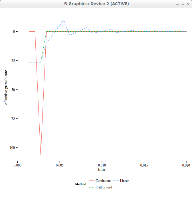
If we simply interpolate the yields linearly intraday, then the yield becomes continuous again, and numerical schemes will work much better.
But if we take a look at the actual curve of “forward” yields, it becomes sawtooth shaped!
effective forward drift used in the finite difference grid with 4 time-steps per day
On the above figure, we can see the Dirac like forward yield if we work with the direct formulas, while interpolating intraday allows to smooth out the initial Dirac overall the interval corresponding to 1-day.
In reality, one should use flat forward interpolation instead, where the forward yield is maintained constant during the day. The forward rate is defined as
where the continuously compounded rate \(r\) is defined so that \(Z(0,t)= e^{-r(t)t}\).
In the case of the Black-Scholes drift, the drift rate is defined so that the forward price (not to confuse with the forward rate) \(F(0,t)= e^{-q(t)t}\).
The flat forward interpolation is equivalent to a linear interpolation on the logarithm of discount factors.
In ACT/365, let \(t_0=\max\left(0,\frac{365}{\left\lceil 365 t \right\rceil-1}\right), t_1 = \frac{365}{\left\lceil 365 t \right\rceil}\), the interpolated yield is:
I moved my blog from blogger to Hugo. Blogger really did not evolve since Google take-over in 2003. Wordpress is today much nicer and prettier. It’s clear that Google did not invest at all, possibly because blogs are passé. Compared to mid 2000, there are very few blogs today. Even programming blogs are scarce. It could be interesting to quantify this. My theory is that it is the direct consequence of the popularity of social networks, and especially facebook (possibly also stackoverflow for programmers): people don’t have time anymore to write as their extra-time is used on social networks. Similarly I noticed that almost nobody comments anymore to the point that even Disqus is very rarely used, and again I attribute that to the popularity of sites like reddit. This is why I did not bother with a comment section on my blog, just email me or tweet about it instead.
I was always attracted by the static web sites concept, because there is actually very little things that ought to be truely dynamic from a individual point of view. Dynamic hosting also tends to be problematic in the long-run, for example I never found the time to upgrade my chord search engine to the newer Google appengine and now it’s just off. I used to freeze my personal website (created with a dynamic templating tool Velocity, django, etc.) with a python script. So a static blog was the next logical step, and these days, it’s quite popular. Static blogs put the author fully in control of the content and its presentation. Jekyll started the trend along with github allowing good old personal websites. It offers a modern looking blog, with very little configuration steps. I tried Hugo instead because it’s written in the Go language. It’s much faster, but I don’t really care about that for something of the size of my blog. I was curious however how good was the Go language on real world projects, and I knew I could always customize it if I ever needed to. Interestingly, I did stumble on a few panics (core dump equivalent where the program just crashes, in this case the hugo local server), something that does not happen with Java based tools or even with Ruby or Python based tools. Even though I like the Go language more and more (I am doing some pet project with it - I believe in the focus on fast compilation and simple language), I found this a bit alarming. This is clearly a result of the errors versus exceptions choice, as it’s up to the programmer to handle the errors properly and not panic unnecessarily (I even wonder if it makes any sense to panic for a server).
Anyway I think it looks better now, maybe a bit too minimalist. I’ll add details when I have more time.