The option chain on Yahoo finance shows an implied volatility number for each call or put option in the last column.
I was wondering a bit how they computed that number. I did not exactly find out their methodology, especially since we don’t even know the daycount convention used, but
I did find that it was likely just garbage.
A red-herring is for example the large discrepancy between put vols and call vols. For example strike 670, call vol=50%, put vol=32%.
This suggests that the two are completely decoupled, and they use some wrong forward (spot price?) to obtain those numbers. If I compute
the implied volatilities using put-call parity close to the money to find out the implied forward price, I end up with ask vols of 37% and 34% or call and put mid vols of 33%.
By considering the put-call parity, I assume European option prices, which is not correct in this case. It turns out however, that with the low interest rates we live in, there is nearly zero additional value due to the American early exercise.
I am not sure what use people can have of Yahoo implied volatilities.
Tufte proposes interesting guidelines to present data, or even to design written semi-scientific papers or books. Some advices
are particularly relevant like the careful use of colors (don’t use all the colors of the rainbow just because you can), and
in general don’t add lines in a graph or designs that are not directly relevant to the message that needs to be conveyed. There is also a parallel
with Feynman message against (Nasa) Powerpoint presentations. But other inspirations, are somewhat doubtful.
He seems to have a fetish for old texts. They might be considered pretty, or interesting in some ways, but
I don’t find them particularly easy to read. They look more like esoteric books rather than practical books. If you want to write
the new Bible for your new cult, it’s probably great, not so sure it’s so great for a more simple subject.
Also somewhat surprisingly, his own website is not very well designed, it looks like a maze and very end of 90s.
I experimented a bit with the Tufte latex template. It produced that document for example. But someone rightfully pointed out to me
that the reference style was not really elegant, that it did not look like your typical nice science paper references. Furthermore,
using superscript so much could be annoying for someone used to read math and consider superscript numbers as math symbols.
In general, there seems to be a conflict between the use of Latex and many Tufte guidelines:
Latex does not encourage you to lay out one by one each piece,
something the good old desktop publishing software allow you to do quite well.
I was also wondering a bit on what design to use for a book. And I realised that the best layout to consider is simply the layout
of a book I enjoyed to read. For example, I like the recent SIAM book design, I find that it gives enough space to read the text
and the maths without having the impression of deciphering some codex, and without headache. It turns out there is even a latex template available.
When the dividend curve is built from discrete cash dividends, the dividend yield is discontinuous at the dividend time as the asset price jumps from the dividend amount.
This can be particularly problematic for numerical schemes like finite difference methods. In deed, a finite difference grid
will make use of the forward yield (eventually adjusted to the discretisation scheme), which explodes then.
Typically, if one is not careful about this, then increasing the number of time steps does not increase accuracy anymore, as
the spike just becomes bigger on a smaller time interval. A simple work-around is to limit the resolution to one day.
This means that intraday, we interpolate the dividend yield.
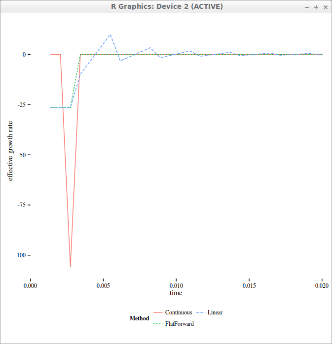
If we simply interpolate the yields linearly intraday, then the yield becomes continuous again, and numerical schemes will work much better.
But if we take a look at the actual curve of “forward” yields, it becomes sawtooth shaped!
effective forward drift used in the finite difference grid with 4 time-steps per day
On the above figure, we can see the Dirac like forward yield if we work with the direct formulas, while interpolating intraday allows to smooth out the initial Dirac overall the interval corresponding to 1-day.
In reality, one should use flat forward interpolation instead, where the forward yield is maintained constant during the day. The forward rate is defined as
where the continuously compounded rate \(r\) is defined so that \(Z(0,t)= e^{-r(t)t}\).
In the case of the Black-Scholes drift, the drift rate is defined so that the forward price (not to confuse with the forward rate) \(F(0,t)= e^{-q(t)t}\).
The flat forward interpolation is equivalent to a linear interpolation on the logarithm of discount factors.
In ACT/365, let \(t_0=\max\left(0,\frac{365}{\left\lceil 365 t \right\rceil-1}\right), t_1 = \frac{365}{\left\lceil 365 t \right\rceil}\), the interpolated yield is:
I moved my blog from blogger to Hugo. Blogger really did not evolve since Google take-over in 2003. Wordpress is today much nicer and prettier. It’s clear that Google did not invest at all, possibly because blogs are passé. Compared to mid 2000, there are very few blogs today. Even programming blogs are scarce. It could be interesting to quantify this. My theory is that it is the direct consequence of the popularity of social networks, and especially facebook (possibly also stackoverflow for programmers): people don’t have time anymore to write as their extra-time is used on social networks. Similarly I noticed that almost nobody comments anymore to the point that even Disqus is very rarely used, and again I attribute that to the popularity of sites like reddit. This is why I did not bother with a comment section on my blog, just email me or tweet about it instead.
I was always attracted by the static web sites concept, because there is actually very little things that ought to be truely dynamic from a individual point of view. Dynamic hosting also tends to be problematic in the long-run, for example I never found the time to upgrade my chord search engine to the newer Google appengine and now it’s just off. I used to freeze my personal website (created with a dynamic templating tool Velocity, django, etc.) with a python script. So a static blog was the next logical step, and these days, it’s quite popular. Static blogs put the author fully in control of the content and its presentation. Jekyll started the trend along with github allowing good old personal websites. It offers a modern looking blog, with very little configuration steps. I tried Hugo instead because it’s written in the Go language. It’s much faster, but I don’t really care about that for something of the size of my blog. I was curious however how good was the Go language on real world projects, and I knew I could always customize it if I ever needed to. Interestingly, I did stumble on a few panics (core dump equivalent where the program just crashes, in this case the hugo local server), something that does not happen with Java based tools or even with Ruby or Python based tools. Even though I like the Go language more and more (I am doing some pet project with it - I believe in the focus on fast compilation and simple language), I found this a bit alarming. This is clearly a result of the errors versus exceptions choice, as it’s up to the programmer to handle the errors properly and not panic unnecessarily (I even wonder if it makes any sense to panic for a server).
Anyway I think it looks better now, maybe a bit too minimalist. I’ll add details when I have more time.
On the Wilmott forum, Pat Hagan has recently suggested to cap the equivalent local volatility in order to control the wings and better match CMS prices. It also helps making the SABR approximation better behaved as the expansion is only valid when
While it is straightforward to include in the PDE, it is more difficult to derive a good approximation. The zero-th order behaves as expected, but the first order formula has a unnatural kink, likely because of the non differentiability due to the min function.
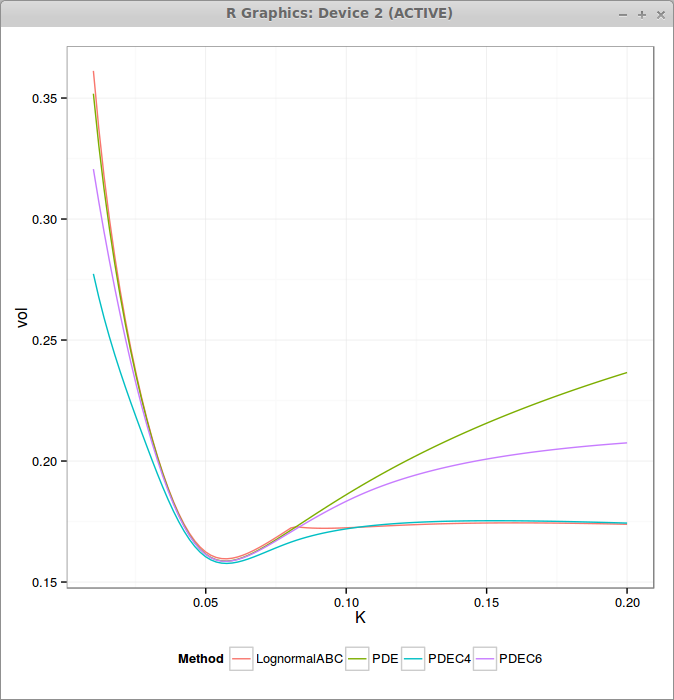
The following graphs presents the non capped PDE, the capped PDE with M=4*nu (PDEC4) and M=6*nu (PDEC6) as well as the approximation (Andersen Ratcliffe / Gatheral first order) where I have only taken care of the right wing. The SABR parameters are alpha = 0.0630, beta = 0.7, rho = -0.363, nu = 0.421, T = 10, f = 0.0439.
We can see that the higher the cap is, the closer we are to the standard SABR PDE, and the lower the cap is, the flatter are the wings.
The approximation matches well ATM (it is then equivalent to standard SABR PDE) but then has a discontinuous derivative for the K that reaches the threshold M. Far away, it matches very well again.
There is something funny going on with upcoming generic top level domains (gTLDs), they seem to be looked up in a strange manner (at least on latest Linux). For example:
ping chrome
or
ping nexus
returns 127.0.53.53.
While existing official gTLDs don't (ping dental returns "unknown host" as expected). I first thought it was a network misconfiguration, but as I am not the only one to notice this, it's likely a genuine internet issue.
I am ambivalent towards David Foster Wallace. He can write the most creative sentences and make innocuous subjects very interesting. At the same time, i never finished his bookInfinite Jest, partly because the characters names are too awkward for me so that i never exactly remember who is who, but also because the story itself is a bit too crazy.
I knew however that a non fiction book on the subject of infinity written by him would make for a very interesting read. And I have not been disappointed. It’s in between maths and philosophy going back to the Greeks up to Gödel through a lot of Cantor following more or less the historical chronology.
Most of it is easy to read and follow, except the last part around sets and transfinite numbers. This last part is actually quite significant as it tries to explain why we still have no satisfying theory around the problems raised by infinity especially in the context of a Sets theory. I did not expect to learn much around the subject, I was disappointed. The book showed me how naive I was and how tricky the concept of infinity can be.
While I found the different explanations around Zeno’s paradox of the arrow very clever, there is one other view possible: the arrow really does not move at each instant (you could think of those as a snapshot) but an interval of time is just not a simple succession of instants. This is not so far of Aristotle attack, but the key here is around what is an interval really. DFW suggests slightly this interpretation as well p144 but it’s not very explicit.
I had not heard about Kronecker’s conception that only integers were mathematically real (against decimals, irrationals, infinite sets). I find it very appropriate in the frame of computer science. Everything ends up as finite integers (a binary representation) and we are always confronted to the process of transforming the continuous, that despite all its conceptual issues is often simpler to reason in to solve concrete problems, to the finite discrete.
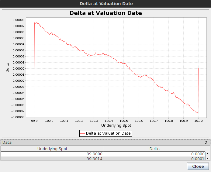
I just stumbled upon this particularly illustrative case where the Crank-Nicolson finite difference scheme behaves badly, and the Rannacher smoothing (2-steps backward Euler) is less than ideal: double one touch and double no touch options.
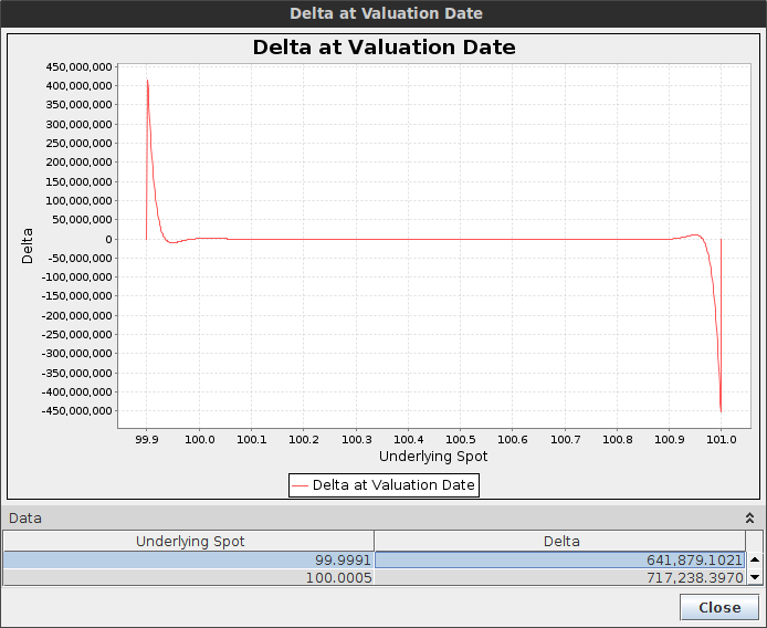
It is particularly evident when the option is sure to be hit, for example when the barriers are narrow, that is our delta should be around zero as well as our gamma. Let's consider a double one touch option with spot=100, upBarrier=101, downBarrier=99.9, vol=20%, T=1 month and a payout of 50K.
Crank-Nicolson shows big spikes in the delta near the boundary
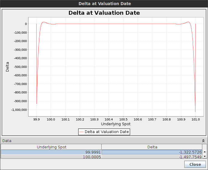
Rannacher shows spikes in the delta as well
Crank-Nicolson spikes are so high that the price is actually a off itself.
The Rannacher smoothing reduces the spikes by 100x but it's still quite high, and would be higher had we placed the spot closer to the boundary. The gamma is worse. Note that we applied the smoothing only at maturity. In reality as the barrier is continuous, the smoothing should really be applied at each step, but then the scheme would be not so different from a simple Backward Euler.
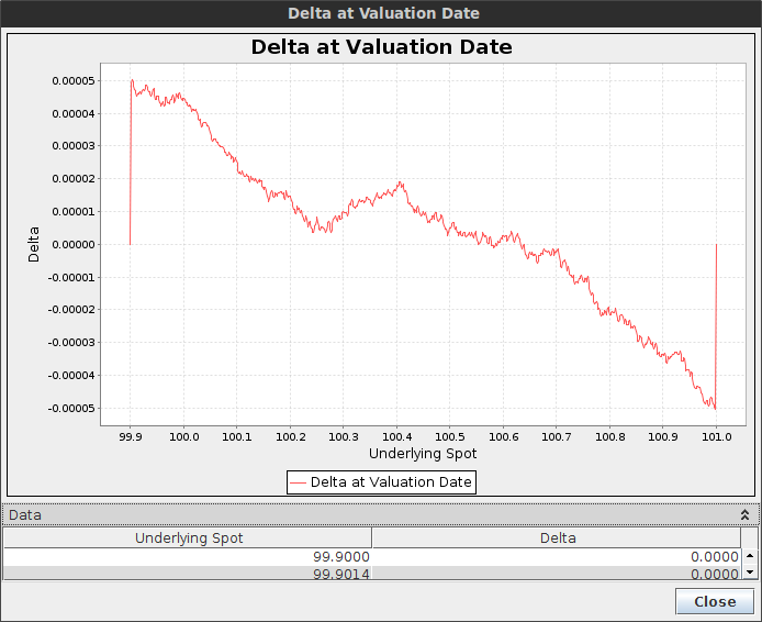
In contrast, with a proper second order finite difference scheme, there is no spike.
Delta with the TR-BDF2 finite difference method - the scale goes from -0.00008 to 0.00008.
Delta with the Lawson-Morris finite difference scheme - the scale goes from -0.00005 to 0.00005
Both TR-BDF2 and Lawson-Morris (based on a local Richardson extrapolation of backward Euler) have a very low delta error, similarly, their gamma is very clean. This is reminiscent of the behavior on American options, but the effect is magnified here.
I was wondering how to generate some nice cloudy like texture with a simple program. I first thought about using the Brownian motion, but of course if one uses it raw, with one pixel representing one movement in time, it's just going to look like a very noisy and grainy picture like this:
Normal noise
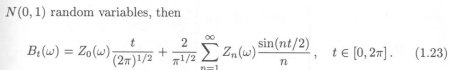
There is however a nice continuous representation of the Brownian motion : the Paley-Wiener representation
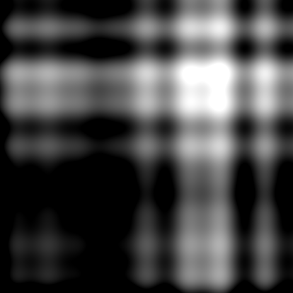
This can produce an interesting smooth pattern, but it is just 1D. In the following picture, I apply it to each row (the column index being time), and then for each column (the row index being time). Of course this produces a symmetric picture, especially as I reused the same random numbers
If I use new random numbers for the columns, it is still symmetric, but destructive rather than constructive.
It turns out that spatial processes are something more complex than I first imagined. It is not a simple as using a N-dimensional Brownian motion, as it would produce a very similar picture as the 1-dimensional one. But this paper has a nice overview of spatial processes. Interestingly they even suggest to generate a Gaussian process using a Precision matrix (inverse of covariance matrix). I never thought about doing such a thing and I am not sure what is the advantage of such a scheme.
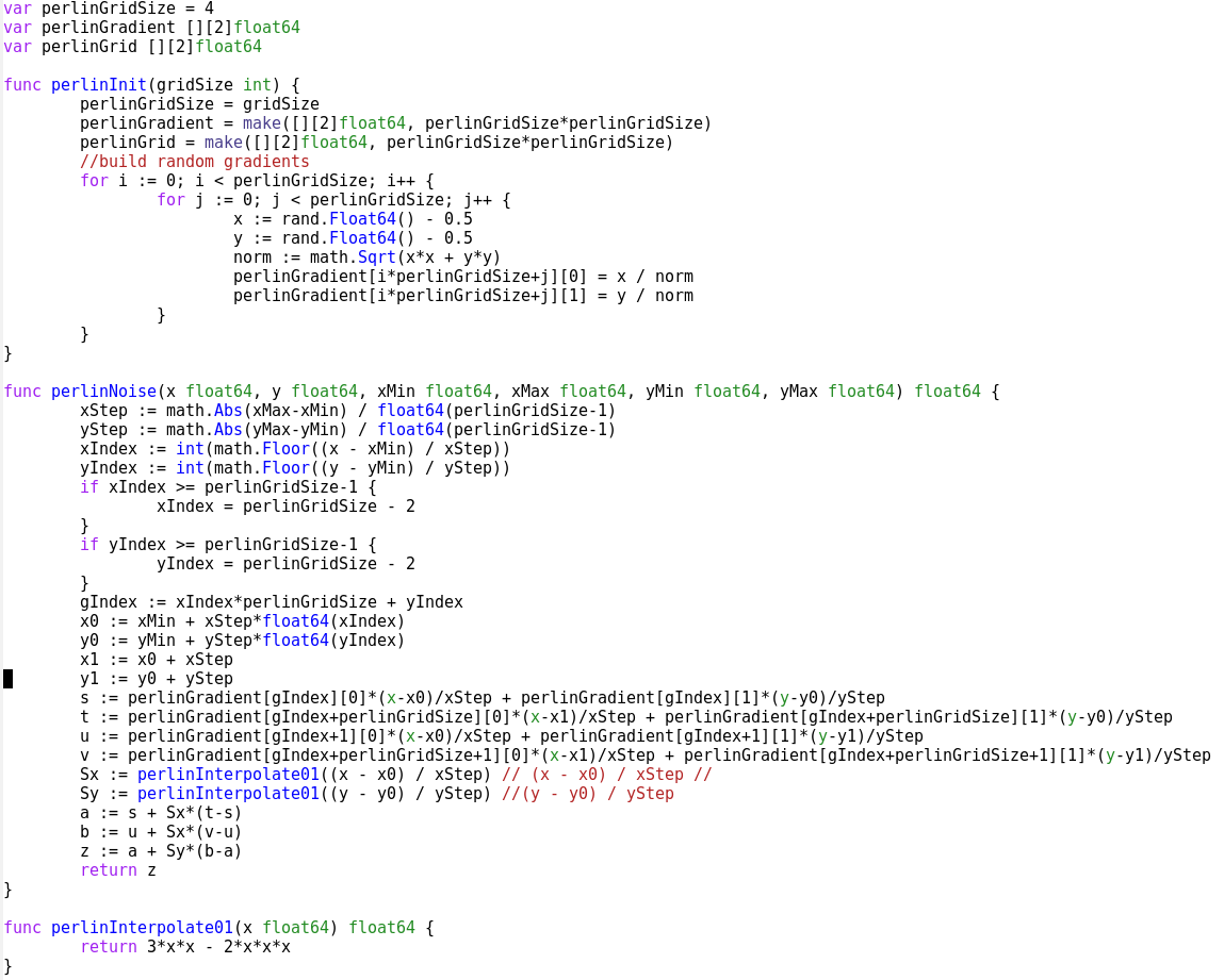
There is a standard graphic technique to generate nice textures, originating from Ken Perlin for Disney, it is called simply Perlin Noise. It turns out that several web pages in the top Google results confuse simple Perlin noise with fractal sum of noise that Ken Perlin also helped popularize (see his slides: standard Perlin noise, fractal noise). Those pages also believe that the later is simpler/faster. But there are two issues with fractal sum of noise: the first one is that it relies on an existing noise function - you need to first build one (it can be done with a random number generator and an interpolator), and the second one is that it ends up being more complex to program and likely to evaluate as well, see for example the code needed here. The fractal sum of noise is really a complementary technique.
The insight of Perlin noise is to not generate random color values that would be assigned to shades of grey as in my examples, but to generate random gradients, and interpolate on those gradient in a smooth manner. In computer graphics they like the cosine function to give a little bit of non-linearity in the colors. A good approximation, usually used as a replacement in this context is 3x^2 - 2x^3. It's not much more complicated than that, this web page explains it in great details. It can be programmed in a few lines of code.
very procedural and non-optimized Go code for Perlin noise
I have looked a few months ago already at Julia, Dart, Rust and Scala programming languages to see how practical they could be for a simple Monte-Carlo option pricing.
I forgot the Go language. I had tried it 1 or 2 years ago, and at that time, did not enjoy it too much. Looking at Go 1.5 benchmarks on the computer language shootout, I was surprised that it seemed so close to Java performance now, while having a GC that guarantees pauses of less 10ms and consuming much less memory.
I am in general a bit skeptical about those benchmarks, some can be rigged. A few years ago, I tried my hand at the thread ring test, and found that it actually performed fastest on a single thread while it is supposed to measure the language threading performance. I looked yesterday at one Go source code (I think it was for pidigits) and saw that it just called a C library (gmp) to compute with big integers. It’s no surprise then that Go would be faster than Java on this test.
So what about my small Monte-Carlo test?
Well it turns out that Go is quite fast on it:
Multipl.
Rust
Go
1
0.005
0.007
10
0.03
0.03
100
0.21
0.29
1000
2.01
2.88
It is faster than Java/Scala and not too far off Rust, except if one uses FastMath in Scala, then the longest test is slighly faster with Java (not the other ones).
There are some issues with the Go language: there is no operator overloading, which can make matrix/vector algebra more tedious and there is no generic/template. The later is somewhat mitigated by the automatic interface implementation. And fortunately for the former, complex numbers are a standard type. Still, automatic differentiation would be painful.
Still it was extremely quick to grasp and write code, because it’s so simple, especially when compared to Rust. But then, contrary to Rust, there is not as much safety provided by the language. Rust is quite impressive on this side (but unfortunately that implies less readable code). I’d say that Go could become a serious alternative to Java.
I also found an interesting minor performance issue with the default Go Rand.Float64, the library convert an Int63 to a double precision number this way:
The reasoning behind this later code is that the mantissa is 52 bits, and this is the most accuracy we can have between 0 and 1. There is no need to go further, this also avoids the issue around 1. It’s also straightforward that is will preserve the uniform property, while it’s not so clear to me that r.Int63()/2^63 is going to preserve uniformity as double accuracy is higher around 0 (as the exponent part can be used there) and lesser around 1: there is going to be much more multiple identical results near 1 than near 0.
It turns out that the if check adds 5% performance penalty on this test, likely because of processor caching issues. I was surprised by that since there are many other ifs afterwards in the code, for the inverse cumulative function, and for the payoff.