Here are the main steps of Hagan derivation. Let's recall his notation for the SABR model where typically, \\(C(F) = F^\beta\\)
First, he defines the moments of stochastic volatility:
Then he integrates the Fokker-Planck equation over all A, to obtain
On the backward Komolgorov equation, he applies a Lamperti transform like change of variable:
And then makes another change of variable so that the PDE has the same initial conditions for all moments:
This leads to
It turns out that there is a magical symmetry for k=0 and k=2.
Note that in the second equation, the second derivative applies to the whole.
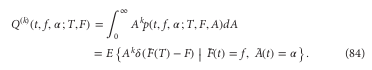
Because of this, he can express \\(Q^{(2)}\\) in terms of \\(Q^{(0)}\\):
And he plugs that back to the integrated Fokker-Planck equation to obtain the arbitrage free SABR PDE:
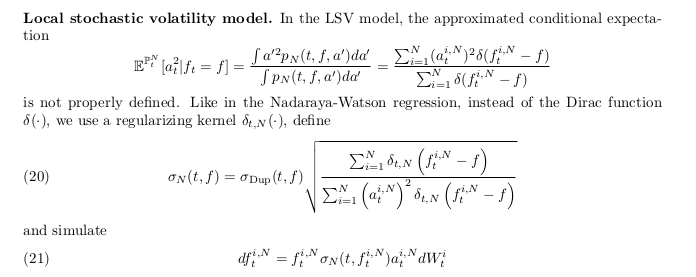
There is a simple more common explanation in the world of local stochastic volatility for what's going on. For example, in the particle method paper from Guyon-Labordère, we have the following expression for the true local volatility.
In the first equation, the numerator is simply \(Q^{(2)}\) and the denominator \(Q^{(0)}\). Of course, the integrated Fokker-Planck equation can be rewritten as:
Karlsmark uses that approach directly in his thesis, using the expansions of Doust for \(Q^{(k)}\). Looking a Doust expansions, the fraction reduces straightforwardly to the same expression as Hagan, and the symmetry in the equations appears a bit less coincidental.