In the Black-Scholes model with a term-structure of volatilities, the Log-Euler Monte-Carlo scheme is not necessarily exact.
This happens if you have two assets \(S_1\) and \(S_2\), with two different time varying volatilities \(\sigma_1(t), \sigma_2(t) \). The covariance from the Ito isometry from \(t=t_0\) to \(t=t_1\) reads $$ \int_{t_0}^{t_1} \sigma_1(s)\sigma_2(s) \rho ds, $$ while a naive log-Euler discretization may use
$$ \rho \bar\sigma_1(t_0) \bar\sigma_2(t_0) (t_1-t_0). $$
In practice, the \( \bar\sigma_i(t_0) \) are calibrated such that the vanilla option prices are exact, meaning
$$ \bar{\sigma}_i^2(t_0)(t_1-t_0) = \int_{t_0}^{t_1} \sigma_i^2(s) ds.$$
As such the covariance of the log-Euler scheme does not match the covariance from the Ito isometry unless the volatilities are constant in time. This means that the prices of European vanilla basket options is going to be slightly off, even though they are not path dependent.
The fix is of course to use the true covariance matrix between \(t_0\) and \(t_1\).
The issue may also happen if instead of using the square root of the covariance matrix in the Monte-Carlo discretization, the square root of the correlation matrix is used.
In my previous blog post, I looked at the roughness of the SVCJ stochastic volatility model with jumps (in the volatility). In this model, the jumps occur randomly, but at discrete times. And with typical parameters used in the litterature, the jumps are not so frequent. It is thus more interesting to look at the roughness of pure jump processes, such as the CGMY process.
The CGMY process is more challenging to simulate. I used the approach based on the characteristic function described in Simulating Levy Processes from Their Characteristic Functions and Financial Applications. Ballota and Kyriakou add some variations based on FFT pricing of the characteristic function in Monte Carlo simulation of the CGMY process and option pricing and pay much care about a proper truncation range. Indeed, I found that the truncation range was key to simulate the process properly and not always trivial to set up especially for \(Y \in (0,1) \). I however did not implement any automated range guess as I am merely interested in very specific use cases, and I used the COS method instead of FFT.
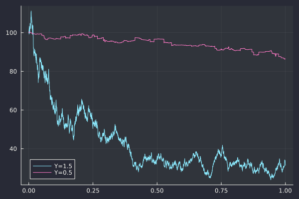
I also directly analyze the roughness of a sub-sampled asset path (the exponential of the CGMY process), and not of some volatility path as I was curious if pure jump processes would mislead roughness estimators. I simulated the paths corresponding to parameters given in Fang thesis The COS Method - An Efficient Fourier Method for Pricing Financial Derivatives: C = 1, G = 5, M = 5, Y = 0.5 or Y = 1.5.
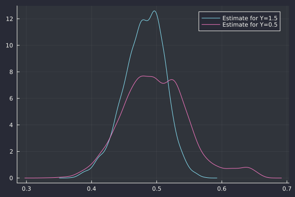
And the corresponding Hurst index estimate via the Cont-Das method:
Similarly the Gatheral-Rosenbaum estimate has no issue finding H=0.5.
I was wondering if adding jumps to stochastic volatility, as is done in the SVCJ model of Duffie, Singleton and Pan “Transform Analysis and Asset Pricing for Affine Jump-Diffusion” also in Broadie and Kaya “Exact simulation of stochastic volatility and other affine jump diffusion processes”, would lead to rougher paths, or if it would mislead the roughness estimators.
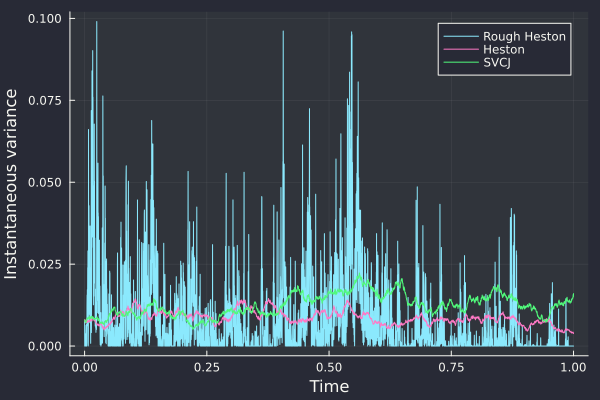
The answer to the first question can almost be answered visually:
The parameters used are the one from Broadie and Kaya: v0=0.007569, kappa=3.46, theta=0.008, rho=-0.82, sigma=0.14 (Heston), jump correlation -0.38, jump intensity 0.47, jump vol 0.0001, jump mean 0.05, jump drift -0.1.
The Rough Heston with H=0.1 is much “noisier”. There is not apparent difference between SVCJ and Heston in the path of the variance.
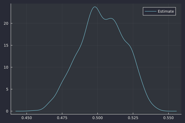
The estimator of Cont and Das (on a subsampled path) leads to a Hurst exponent H=0.503, in line with a standard Brownian motion.
Cont-Das estimate H=0.503.
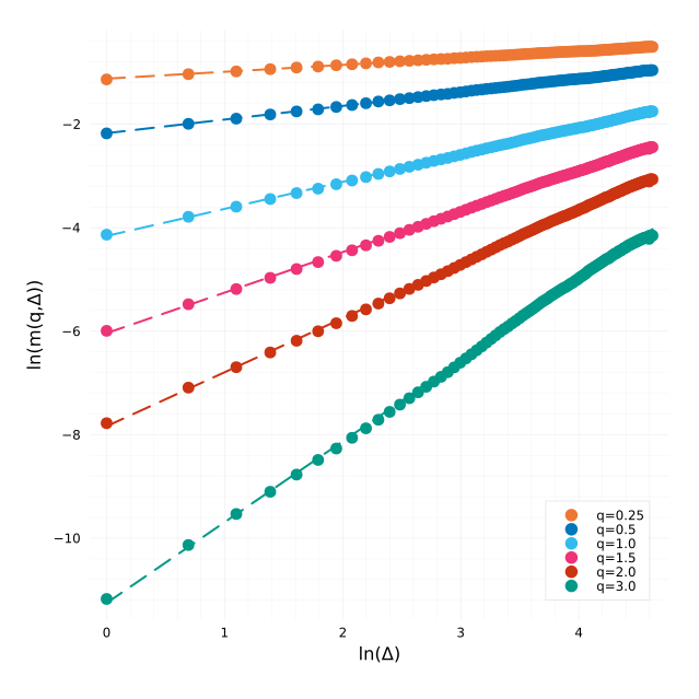
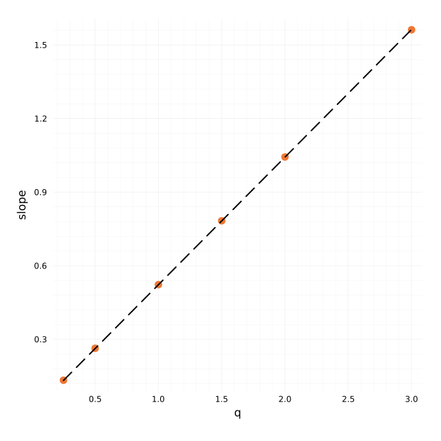
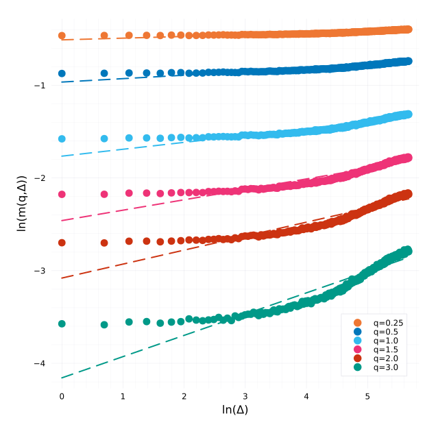
The estimator from Rosenbaum and Gatheral leads to a Hurst exponent (slope of the regression) H=0.520 with well behaved regressions:
Regressions for each q.
Regression over all qs which leads to the estimate of H.
On this example, there are relatively few jumps during the 1 year duration. If we multiply the jump intensity by 1000 and reduce the jump mean accordingly, the conclusions are the same. Jumps and roughness are fundamentally different.
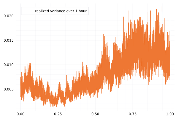
Of course this does not mean that the short term realized volatility does not look rough as evidenced in Cont and Das paper:
The 1 hour realized volatility looks rough.
I computed the realized volatility on a subsampled path, using disjoint windows of 1h of length.
It is not really rough, estimators will have a tough time leading to stable estimates on it.
Hurst exponent estimation based on the 1h realized variance. The mean H=0.054 but is clearly not reliable.
This is very visible with the Rosenbaum-Gatheral way of estimating H, we see that the observations do not fall on a line at all but flatten:
Regressions for each q based on the 1h realized variance.
The pure Heston model leads to similar observations.
I received a few e-mails asking me for the code I used to measure roughness in my preprint on the roughness of the implied volatility. Unfortunately, the code I wrote for this paper is not in a good state, it’s all in one long file line by line, not necessarily in order of execution, with comments that are only meaningful to myself.
In this post I will present the code relevant to measuring the oxford man institute roughness with Julia. I won’t go into generating Heston or rough volatility model implied volatilities, and focus only on the measure on roughness based on some CSV like input. I downloaded the oxfordmanrealizedvolatilityindices.csv from the Oxford Man Institute website (unfortunately now discontinued, data bought by Refinitiv but still available in some github repos) to my home directory
using DataFrames, CSV, Statistics, Plots, StatsPlots, Dates, TimeZones
df = DataFrame(CSV.File("/home/fabien/Downloads/oxfordmanrealizedvolatilityindices.csv"))
df1 = df[df.Symbol.==".SPX",:]
dsize = trunc(Int,length(df1.close_time)/1.0)
tm = [abs((Date(ZonedDateTime(String(d),"y-m-d H:M:S+z"))-Date(ZonedDateTime(String(dfv.Column1[1]),"y-m-d H:M:S+z"))).value) for d in dfv.Column1[:]];
ivm = dfv.rv5[:]
using Roots, Statistics
function wStatA(ts, vs, K0,L,step,p)
bvs = vs # big.(vs) bts = ts # big.(ts) value = sum( abs(log(bvs[k+K0])-log(bvs[k]))^p / sum(abs(log(bvs[l+step])-log(bvs[l]))^p for l in k:step:k+K0-step) * abs((bts[k+K0]-bts[k])) for k=1:K0:L-K0+1)
return value
endfunction meanRoughness(tm, ivm, K0, L)
cm = zeros(length(tm)-L);
for i =1:length(cm)
local ivi = ivm[i:i+L]
local ti = tm[i:i+L]
T = abs((ti[end]-ti[1]))
try cm[i] =1.0/ find_zero(p -> wStatA(ti, ivi, K0, L, 1,p)-T,(1.0,100.0))
catch e
ifisa(e, ArgumentError)
cm[i] =0.0else throw(e)
endendend meanValue = mean(filter( function(x) x >0end,cm))
stdValue = std(filter( function(x) x >0end,cm))
return meanValue, stdValue, cm
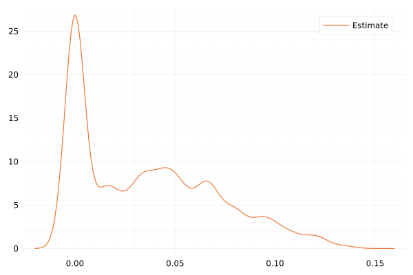
endmeanValue, stdValue, cm = meanRoughness(tm, ivm, K0,K0^2)
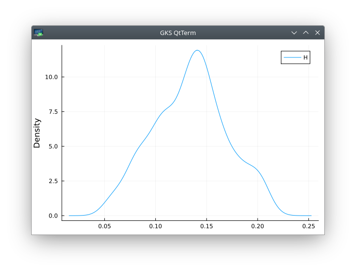
density(cm,label="H",ylabel="Density")
The last plot should look like
It may be slightly different, depending on the date (and thus the number of observations) of the CSV file (the ones I found on github are not as recent as the one I used initially in the paper).
I was experimenting with the recent SABR basket approximation of Hagan. The approximation only works
for the normal SABR model, meaning beta=0 in SABR combined with the Bachelier option formula.
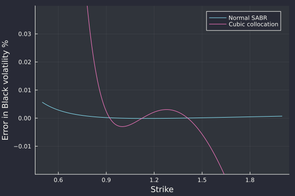
I was wondering how good the approximation would be for two flat smiles (in terms of Black volatilities). I then noticed something that escaped me before: the normal SABR model is able to fit the pure Black model (with constant vols) extremely well. A calibration near the money stays valid very out-of-the-money and the error in Black volatilities is very small.
For very low strikes (25%) the error in vol is below one basis point. And in fact, for a 1 year option of vol 20%, the option value is extremely small: we are in deep extrapolation territory.
It is remarkable that a Bachelier smile formula with 3 free parameters can fit so well the Black vols. Compared to stochastic collocation on a cubic polynomial (also 3 free parameters), the fit is 100x better with the normal SABR.
Error in fit against 10 vanilla options of maturity 1 year and volatility 20% within strike range [0.89, 1.5] .
The Clenshaw-Curtis quadrature is known to be competitive with Gauss quadratures. It has several advantages:
the weights are easy and fast to compute.
adaptive / doubling quadratures are possible with when the Chebyshev polynomial of the second kind is used for the quadrature.
the Chebyshev nodes may also be used to interpolate some costly function.
The wikipedia article has a relatively detailed description on how to compute the quadrature weights corresponding to the Chebyshev polynomial of the second kind (where the points -1 and 1 are included), via a type-I DCT. It does not describe the weights corresponding to the Chebyshev polynomials of the first kind (where -1 and 1 are excluded, like the Gauss quadratures). The numbersandshapes blog post describes it very nicely. There are some publications around computation of Clenshaw-Curtis or Fejer rules, a recent one is Fast construction of Fejér and Clenshaw–Curtis rules for general weight functions.
I was looking for a simple implementation of the quadrature or its weights, leveraging some popular FFT library such as fftw (The Fastest Fourier Transform in the West). I expected it to be a simple search. Instead, it was surprisingly difficult to find even though the code in Julia consists only in a few lines:
chebnodes(T, n::Int) =@. (cos(((2:2:2n) -1) * T(pi) /2n))
x = chebnodes(Float64, N)
m = vcat(sqrt(2), 0.0, [(1+ (-1)^k) / (1- k^2) for k =2:N-1])
ws = sqrt(2/ N) * idct(m)
Second kind (the classic Clenshaw-Curtis, following some article from Treffenden)
cheb2nodes(T, n::Int) =@. (cos(((0:n-1)) * T(pi) / (n-1)))
x = cheb2nodes(Float64, N)
c = vcat(2, [2/ (1- i^2) for i =2:2:(N-1)]) # Standard Chebyshev momentsc = vcat(c, c[Int(floor(N /2)):-1:2]) # Mirror for DCT via FFT ws = real(ifft(c)) # Interior weightws[1] /=2ws = vcat(ws, ws[1]) # Boundary weights
There are some obvious possible improvements: the nodes are symmetric and only need to be computed up to N/2, but the above is quite fast already. The Julia package FastTransforms.jl provides the quadrature weights although the API is not all that intuitive:
Interestingly the first kind is twice faster with FastTransforms, which suggests a similar symetry use as for the second kind. But the second kind is nearly twice slower.
Although Clenshaw-Curtis quadratures are appealing, the Gauss-Legendre quadrature is often slightly more accurate on many practical use cases and there exists also fast enough ways to compute its weights. For example, in the context of a two-asset basket option price using a vol of 20%, strike=spot=100, maturity 1 year, and various correlations we have the below error plots
Correlation = -90%,-50%,50%,90% from top to bottom.
During my vacation, I don’t know why, but I looked at some stability issue with ghost points and the explicit method. I was initially trying out ghost points with the explicit runge kutta Chebyshev/Legendre/Gegenbauer technique and noticed some explosion in some cases.
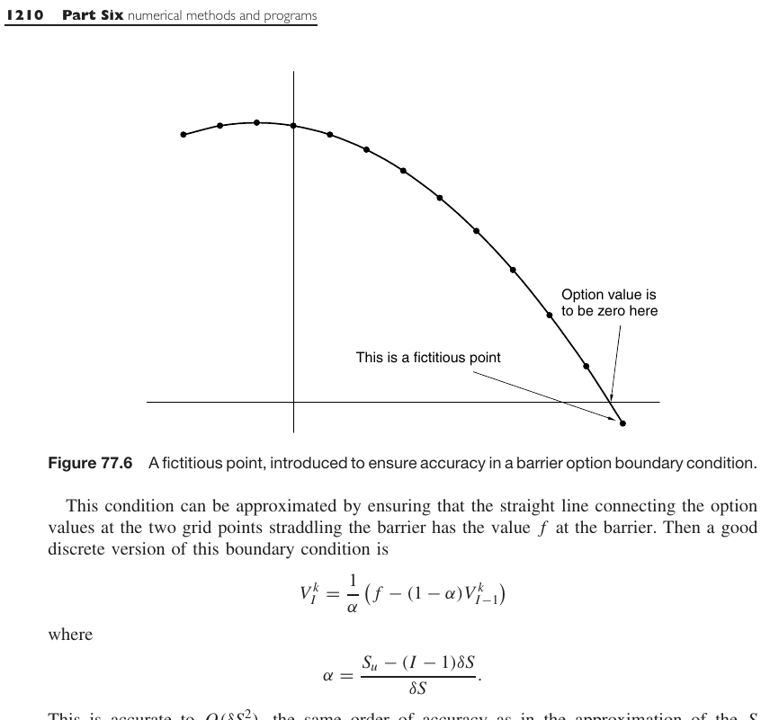
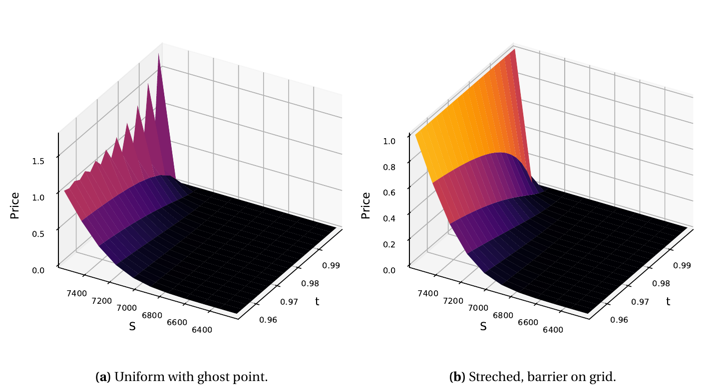
I cornered it down to a stability issue of the standard explicit Euler method with ghost (or fictitious) points. The technique is described in the book “Paul Wilmott on Quantitative Finance” (also in Paul Wilmott introduces quantitative finance), which I find quite good, although I have some friends who are not much fond of it. The technique may be used to compute the price of a continuously monitored barrier option when the barrier does not fall on the grid, or more generally for time-dependent barriers. I however look at it in the simple context of a constant barrier in time.
The ghost point technique (from Paul Wilmott on Quantitative Finance).
I found out that the explicit Euler scheme is unstable if we let the grid boundaries be random. In practice, for more exotic derivatives, the grid upper bound will typically be based on a number of standard deviations from the spot or from the strike price. The spot price moves continually, and the strike price is fairly flexible for OTC options. So the upper bound can really be anything and the explicit Euler may require way too many time-steps to be practical with the ghost point technique. This is all described in the preprint Instabilities of explicit finite difference schemes with ghost points on the diffusion equation.
What does this mean?
The ghost point technique is not appropriate for the explicit Euler scheme (and thus for the Runge-Kutta explicit schemes as well), unless the ghost point is fixed to be in the middle of the grid, or on the grid outside by one space-step. This means the grid needs to be setup in a particular fashion. But if we need to setup the grid such that the barrier falls exactly somewhere then, for a constant barrier option, no ghost point is needed, one just need to place the barrier on the grid and use a Dirichlet boundary condition.
Explicit scheme requires a very large number of time-steps.
Crank_Nicolson oscillations near maturity with the ghost point.
The paper The Moment Formula for Implied Volatility at Extreme Strikes by Roger Lee redefined how practioners extrapolate the implied volatility, by showing that the total implied variance can be at most linear in the wings, with a slope below 2.
Shortly after, the SVI model of Jim Gatheral, with its linear wings, started to become popular.
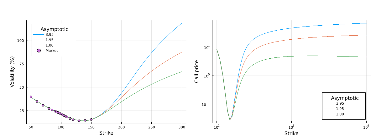
In a recent paper in collaboration with Winfried Koller, we show that the asymptotic bounds are usually overly optimistic. This is somewhat expected, as the bound only holds as the log-moneyness goes to infinity. What is less expected, is that, even at very large strikes (nearly up to the limit of what SVI allow numerically), we may happen to have arbitrages, even though the bounds are respected.
In practice, this manifests by increasing call option prices far away in the wings (increasing call prices are an arbitrage opportunity), which could be problematic for any kind of replication based pricing, such as variance swap pricing.
Increasing call prices for various calibrated SVI parameters respecting the asymptotic boundary constraints.
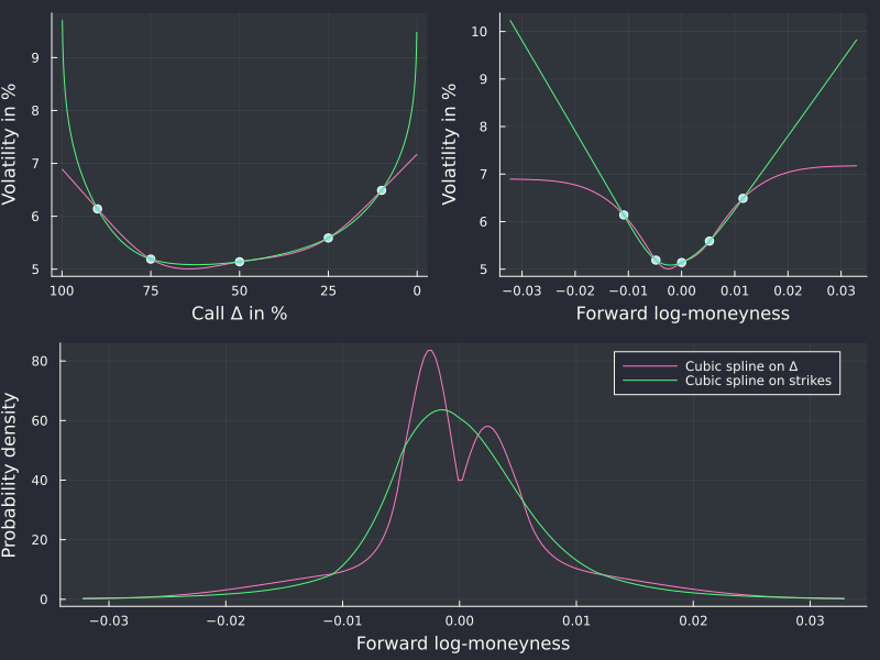
In a Wilmott article from 2018 (Wilmott magazine no. 97) titled “Arbitrage in the perfect volatility surface”, Uwe Wystup points out some interesting issues on seemingly innocuous FX volatility surfaces:
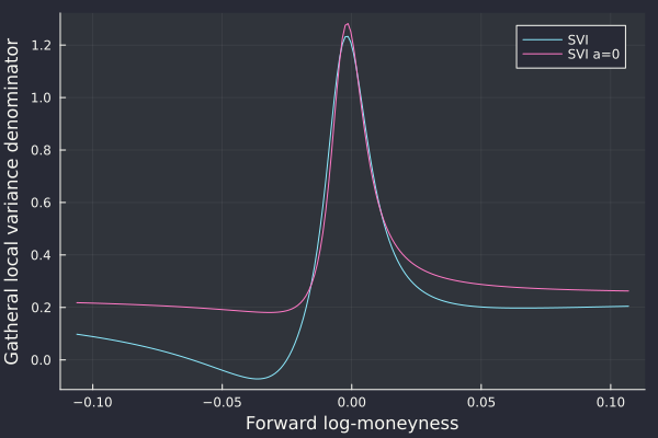
a cubic spline tends to produce artificial peaks/modes in the density.
SVI not arbitrage-free even on seemingly trivial input.
The examples provided are indeed great and the remarks very valid. There is more to it however:
a cubic spline on strikes or log-moneyness does not produce the artificial peak.
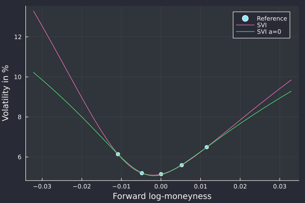
SVI with a=0 is arbitrage-free on this example.
For the first point, the denominator of the Dupire formula in terms of the representation of total variance as a function of logmoneyness gives some clues as it constitues a vega scaled version of the probability density
with direct link to the total variance and its derivatives. In particular it is a simple function of its value, first and second derivatives, without involving any non-linear function and the second derivative only appears as a linear term. As such a low order polynomial representation of the variance in log-moneyness may be adequate.
In contrast, the delta based representation introduces a strong non-linearity with the cumulative normal distribution function.
Splines on AUD/NZD 1w options.
For the second point, it is more of a curiosity. Everybody knows that SVI is not always arbitrage-free and examples of arbitrages abound. Finding such a minimal example is
nice. I noticed that many of the real life butterfly spread arbitrages are avoided if we follow Zeliade’s recommendation to set a >= 0, where a is the base ordinate parameter of SVI.
Yes the fit is slightly worse, but the increased calibration robustness and decrease of the number of smiles with arbitrage is probably worth it.
SVI on AUD/NZD 1w options.
SVI on AUD/NZD 1w options.
Even if I am no particular fan of SVI or of the cubic spline to represent implied volatilities, the subject merited some clarifications.
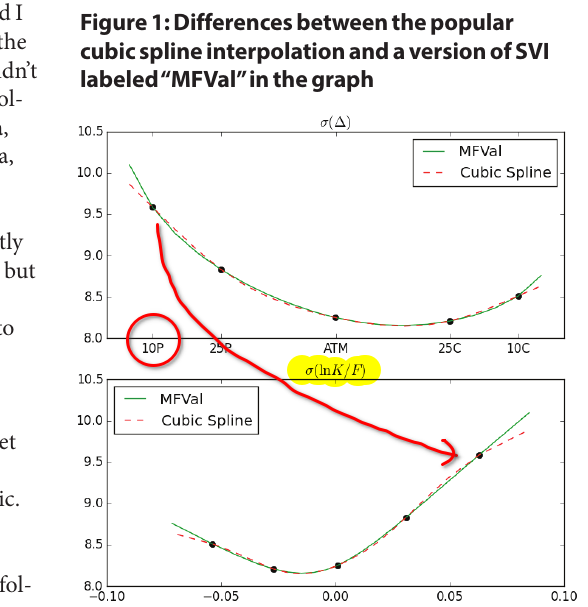
extract of the Wilmott article.
There is a third point which I found quite surprising. The axis is inconsistent between the first two plots of Figure 1. 10 delta means that we are out of the money.
For a call, the strike is thus larger than the forward, and thus the corresponding log-moneyness must be positive. But on the Figure, the 10 Delta call volatility of the first plot does not correspond to the highest log-moneyness point of the second plot.
One of the axis is reversed. This is particularly surprising for an expert like Uwe.
Ooohhhh!
It is reassuring that this kind of mistakes also happen to the best. Every FX quant has Uwe Wystup’s book, next to the Clark and the Castagna.
I recently presented my latest published paper On the Bachelier implied volatility at extreme strikes at the Princeton Fintech and Quant conference.
The presenters were of quite various backgrounds. The first presentations were much more business oriented with lots of AI keywords, but relatively little technical content while the last presentation was
about parallel programming. Many were a pitch to recruit to employees.
The diversity was interesting: it was refreshing to hear about quantitative finance from vastly different perspectives. The presentation from Morgan Stanley about their scala annotation framework to ease up
parallel programming was enlightening. The main issue they were trying to solve is the necessity for all the boilerplate code to handle concurrency, caching, robustness, which obfuscates significantly the business logic in the code.
This is an old problem. Decades ago, rule engines were the trend for similar reasons. Using the example of pricing bonds, the presenters put very well forward the issues in evidence, issues that I found
very relevant.
While writing my own presentation, I realized I had not tried to plot the Bachelier implied volatility fractals. The one corresponding to the Householder method is pretty, and not too far off from
the Black-Scholes case, possibly because the first, second and third derivatives towards the vol are similar between the two models.
Iterations of the Householder method on the problem of solving the Bachelier implied volatility for a given strike and maturity. Each point corresponds to an initial guess in the complex plane.
Of course, this is purely for the fun as this has no practical importance, since we can invert the Bachelier price with near machine accuracy through a fast analytic formula.