As described on wikipedia, a quadratic programming problem with n variables and m constraints is of the form
$$ \min(-d^T x + 1/2 x^T D x) $$ with the
constraints \( A^T x \geq b_0 \), were \(D\) is a \(n \times n\)-dimensional real symmetric matrix, \(A\) is a \(n \times m\)-dimensional real matrix, \( b_0 \) is a \(m\)-dimensional vector of constraints, \( d \) is a \(n\)-dimensional vector, and the variable \(x\) is a \(n\)-dimensional vector.
Solving convex quadratic programming problems happens to be useful in several areas of finance. One of the applications is to find the set of arbitrage-free option prices closest to a given set of market option prices as described in An arbitrage-free interpolation of class C2 for option prices (also published in the Journal of Derivatives). Another application is portfolio optimization.
In a blog post dating from 2018, Jherek Healy found that the sparse solve_qp solver of scilab was the most efficient across various open-source alternatives. The underlying algorithm is actually Berwin Turlach quadprog, originally coded in Fortran, and available as a R package. I had used this algorithm to implement the techniques described in my paper (and even proposed a small improvement regarding machine epsilon accuracy treatment, now included in the latest version of quadprog).
Julia, like Python, offers several good convex optimizers. But those support a richer set of problems than only the basic standard quadratic programming problem. As a consequence, they are not optimized for our simple use case. Indeed, I have ported the algorithm to Julia, and found out a 100x performance increase over the COSMO solver on the closest arbitrage-free option prices problem. Below is a table summarizing the results (also detailed on the github repo main page).
In the context of my thesis, I explored the use of stochastic collocation to capture the marginal densities of a positive asset.
Indeed, most financial asset prices must be non-negative. But the classic stochastic collocation towards the normally distributed random variable, is not.
A simple tweak, proposed early on by Grzelak, is to assume absorption and use the put-call parity to price put options (which otherwise depend on the left tail).
This sort of works most of the time, but a priori, there is no guarantee that we will end up with a positive put option price.
As an extreme example, we may consider the case where the collocation price formula leads to \(V_{\textsf{call}}(K=0) < f \) where \(f \) is the forward price to maturity.
The put-call parity relation applied at \(K=0 \) leads to \(V_{\textsf{put}}(K=0) = V_{\textsf{call}}(K=0)-f < 0 \). This means that for some strictly positive strike, the put option price will be negative, which is non-sensical.
In reality, it thus implies that absorption must happen earlier, not at \(S=0 \), but at some strictly positive asset price. And then it is not so obvious to chose the right value in advance.
In the paper, I look at alternative ways of expressing the absorption, which do not have this issue. Intuitively however, one may wonder why we would go through the hassle of considering a distribution which may end up negative to model a positive price.
In finance, the assumption of lognormal distribution of price returns is very common. The most straighforward would thus be to collocate towards a lognormal variate (instead of a normal one), and use an increasing polynomial map from \([0, \infty) \) to \([0, \infty) \).
There is no real numerical challenge to implement the idea. However it turns out not to work well, for reasons explained in the paper, one of those being a lack of invariance with regards to the lognormal distribution volatility.
This did not make it directly to the final thesis, because it was not core to it. Instead, I explore absorption with the Heston driver process (although, in hindsight, I should have just considered mapping 0 to 0 in the monotonic spline extrapolation). I recently added the paper on the simpler case of positive collocation with a normal or lognormal process to the arxiv.
Steven Koonin, who was Secretary for Science, Department of Energy, in the Obama administration recently wrote a somewhat controversial book on climate science with the title Unsettled. I was curious to read what kind of critics a physicist who partly worked in the field had, even if I believe that climate warming is real, and humans have an influence on it. It turns out that some of his remarks regarding models are relevant way beyond climate science, but some other subjects are not as convincing.
The first half of the book explains how the influence of humans on climate is not as obvious as what many graphs suggest, even those published by well known groups such as CSSR or IPCC.
A recurring theme is plots presented without context/with the wrong context. Many times, when we extend the time span in the past, a very different picture emerges of cyclic variations with cycles of different lengths and amplitudes. Other times, the choice of measure is not appropriate. Yey another aspect is the uncertainty of the models, which seems too rarely discussed in reports/papers, as well as the necessary model parameters tweaking.
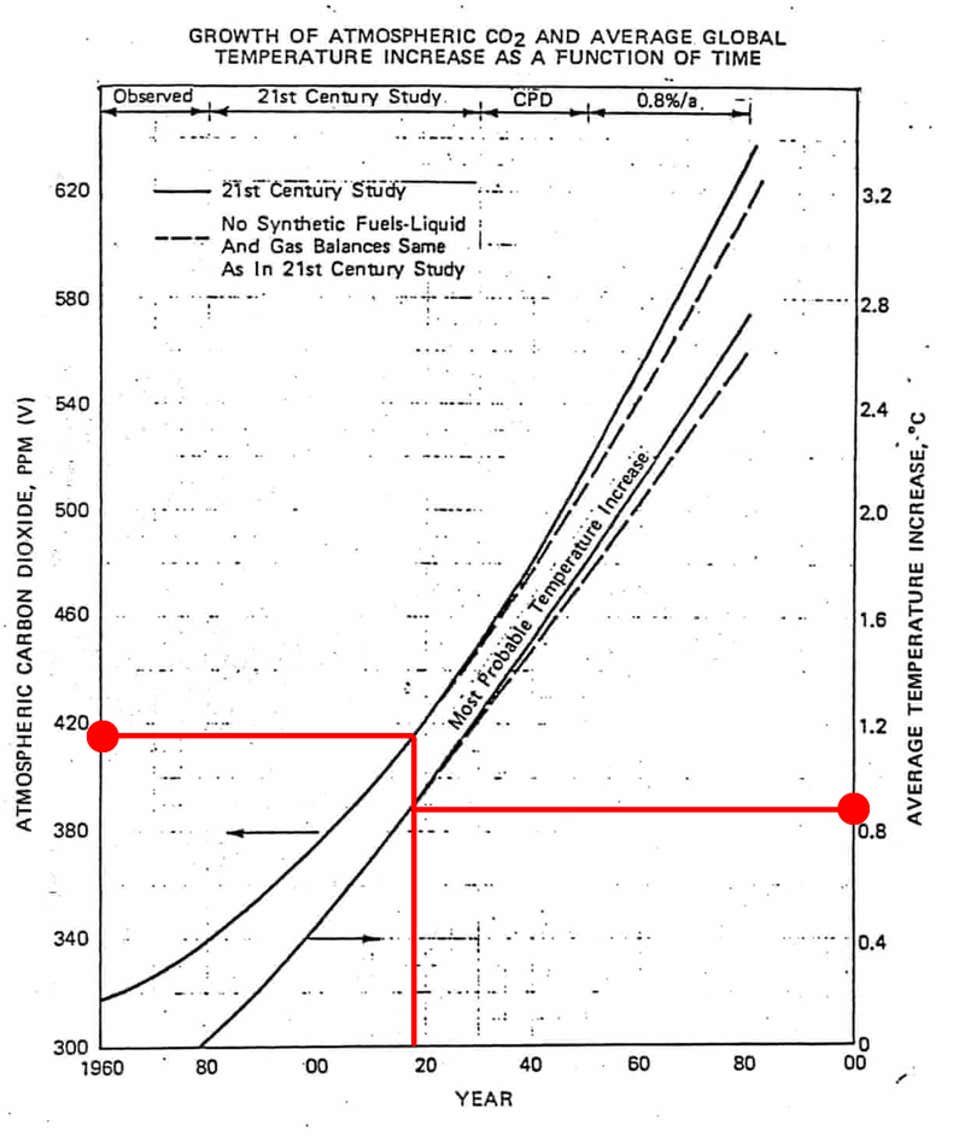
When it comes to CO2, Koonin explains that the decrease in cooling power is much much lower from 400ppm to 800ppm than from 0ppm to 400ppm, because, at 400ppm (the 2019 average) most of the light frequencies are already absorbed. The doubling corresponds only to a 0.8% change in heat intercepting. 1% is however not so small, as it corresponds to 3 degrees Kelvin/Celcius variation. Furthermore, while humans may increase warming with greenhouse gas, they also increase cooling via aerosols, the latter being much less well known and measured (with those taken into account, we arrive at the 1 degree Celcius impact). The author also presents some plots on CO2 on a scale of millions of years to explain that we live in an era of low CO2 ppm. While an interesting fact, this may be a bit misleading since, if we look at at up to 800,000 years back, the CO2 concentration stayed between 200 and 250 ppm, with an explosion only in the recent decades. The climate.gov website provides more context around the latter plot:
In fact, the last time the atmospheric CO₂ amounts were this high was more than 3 million years ago, when temperature was 2°–3°C (3.6°–5.4°F) higher than during the pre-industrial era, and sea level was 15–25 meters (50–80 feet) higher than today.
On this plot, the relation between the temperature increase and the CO2 ppm looks linear, which would be somewhat more alarming.
The conclusion from the first half of the book may be summarized as follows: while climate warming is real, it is not so obvious how much of it is due to humans. The author agrees for maybe around 1 degree Celcius, and suggests it is not necessarily accelerating. The causes are much less clear. There are some interesting subtleties: temperature increases in some places and decreases in others; around cities, the increase mostly due to the expansion of cities (more buildings).
I found the second half to be in contradiction with the first half, although it is clearly not the author’s intent: the second half focuses on how to address humans influence on the climate, and several times, suggests a strong influence of humans emissions on the climate, while the first half of the book was all about minimizing that aspect. This is especially true for carbon emissions, where it is suggested in the first half that additional emisssions will have a comparatively small impact.
The overall message is relatively simple: reducing emissions won’t help much as concentration will only increase in the coming decades (but then wouldn’t it perhaps be so bad to think beyond the coming decades?). Also the scales of emission reductions necessary for a minimum increase (2 degrees) is not realistic at all in the world we live in. Instead, we’d be better off trying to adapt.
Overall, the author denounce the issue of scientific integrity, which is too often absent or not strongly present enough. Having reviewed many papers, and published some in specialized journals, I can’t say I am surprised. Peer review is important, but perhaps not good enough by itself, especially in the short run. Over decades, I think the system may autocorrect itself however.
Github recently moved to support only ssh access via public/private keys. As I use github to host this blog, I was impacted.
The setup on Linux is not very complicated, and relatively well documented on Github itself but all the steps are not listed in a simplistic manner, and some Google search is still required to find out how to setup multiple private keys for various different servers or different repos.
Here is my short guide. In bash, do the following:
ssh-keygen -t ed25519 -C "your_email@example.com"
Make sure to give a specific name, e.g. /home/you/.ssh/id_customrepo_ed25519
One thing that motivated me for vaccination is the fake news propaganda against the Covid-19 vaccines.
A mild example relates to the data from Israel about the delta variant. This kind of article, with the title “Covid 19 Case Data in Israel, a Troubling Trend”, puts emphasis on the doubts on the effectivness of the vaccine:
the vaccine appears to have a negligible effect on an individual as to whether he/she catches the current strain. Moreover, the data indicates that the current vaccines used (Moderna, Pfizer-BioNTech, AstraZeneca) may have a decreasing effect on reduced hospitalizations and death if one does get infected with the Delta variant.
CNBC (far from the best news site) is much more balanced and precise in contrast:
However, the two-dose vaccine still works very well in preventing people from getting seriously sick, demonstrating 88% effectiveness against hospitalization and 91% effectiveness against severe illness, according to the Israeli data published Thursday.
Much more shocking is a tweet from Prashant Bhushan (whoever that is) which was relayed widely enough that I got to see it
Public Health Scotland have revealed that 5,522 people have died within twenty-eight days of having a Covid-19 vaccine within the past 6 months in Scotland alone! This is 9 times the people who died due to Covid from March 2020 till Jan 2021 in Scotland!
It points to an article in the Daily Expose (worse than a tabloid?) with a link to the actual study. Giving an actual link to the source is a very good practice, even if in this case, the authors of the news article write a lengthy text which says the opposite as the paper they cite as being the source. Indeed, p.27 of the paper says
Using the 5-year average monthly death rate (by age band and gender) from 2015 to 2019 for comparison, 8,718 deaths would have been expected among the vaccinated population within 28 days of receiving their COVID-19 vaccination.
This means the observed number of deaths is lower than expected compared with mortality rates for the same time period in previous years…
Why do people write such fake news articles?
I can imagine 3 kinds of motivations:
The author wants to make money/be famous. Writing controversial things, even if completely false, seems to work wonder to attract readership, as long as there is a trend of readers curious about this controverse. The author will gather page views and followers easily, which he may then monetize.
The author is just someone so convinced in his beliefs that everything is interpreted through a very narrow band-pass filter. They will read and pay attention only to the words in the text that will validate their beliefs and forget everything else. I know examples (not on this particular subject) in my own family.
Farm trolls. There are many farm trolls (we always hear of the Russian farm trolls, but they really exist in most countries), where people are paid to spread disinformation on social media. A simple example is the fake reviews on Amazon. Sometimes the goal is to promote a particular political party ideas. Sometimes this political party is financed by a foreign country with specific interests.
The third motivation may act as an amplifier of the first two.
Why are fake news successful?
People do not trust the official government message. On the coronavirus, the French government was initially quite bad at presenting the situation, with the famous “masks are useless” (because they did not have any stock), a couple of months before enforcing masks everywhere. Too many decisions are purely political. A good example is the policy to close a school class on a single positive test when the full school is being tested for coronavirus. The false positive rate guarantees that at least 1/3 of the classes will close. Initially the policy was 3 positive tests, which was much more rational, but not as obvious to understand for the masses. My son ended up being one of those false positives, and it wasn’t a particularly nice experience.
People do not trust traditional media anymore. As the quality of standard newspapers dwindled with the rise of the internet, people do not trust those much anymore. Also, perhaps fairly, it is not clear if classic tradional media present better news than free modern social media. There are exceptions of course (typically with monthly publications).
Social media bias: almost all social networks act as narrow band-pass filter. If you look at one video of cat on youtube, you will end up with videos of cats in your youtube frontpage every day. Controversial subjects/videos are given a considerable space. A main reason for this behavior is that they are optimized for page views/to attract your attention.
Generalized attention deficit disorder due to the ubiquity of smart phones. Twitter got famous because of the 127 characters message limit. Newspaper articles are perhaps five times shorter than they used to be in the early 1990s. The time we have is limited and a lot of it is spent reading/writing short updates to various Whatsapp groups or other social network apps.
Conclusion
This was not the only motivator, another strong one is a Russian friend who caught the Covid-19 in July 2021, who was not very pro-vaccination, but thought, once it was too late, “I really should have applied for the vaccine”, as he realized it impacted the whole circle of relations around him. Then, one by one, his whole family caught the Covid. Fortunately, no-one died.
After several weeks, my parents and I were finally able to have a real world meeting with the advisor at the bank. The advisor is a young woman with an obvious background in sales.
In order to process the paperwork around the reimbursement of the phishing scam, the main issue was the request of the original phishing e-mail by the bank, as my mother had deleted the e-mail. It turns out, that in Thunderbird, deleted e-mails are not deleted on disk until an operation of compactification of the mailbox is done. I was thus able to recover the deleted e-mail. Interestingly, the deleted e-mail was not in the trash file, but directly in the inbox file.
At first, I sent the message source as PDF, along with a screenshot to the bank. The bank asked to forward the e-mail instead. Interestingly, it turns out that once a phishing e-mail is registered in the various anti-phishing filters, it is not possible to forward (directly or in attachment) or copy paste the email as most servers (including the bank servers) will detect the new email as potential phishing and directly reject the e-mail (reject error).
So the standard process of the bank is not really appropriate. It can be followed only during the very short period (more luck than anything) where the phishing has not yet been registered in the anti-phishing filters. I noticed by a simple Google search that many other institution follow a similar process, where they ask to forward the phishing e-mail to a specific e-mail address.
The good news so far is that officially, the advisor pushed the fraud case forward, although it is not entirely clear at this point if it will be processed properly. What shocked me more was the speech of the bank advisor. First, she scared us by telling stories of various credit card frauds (obviously not related to our bank credentials fraud). When she mentioned insurances against credit card frauds, without selling them yet to us, her goal became clear. Then she thought comforting that this kind of fraud only happens once, because once you are confronted to a fraud, you would then be more careful and not make the same mistake anymore, not a convincing argument at all in my views. She indirectly kept blaming my mother for entering her credentials, but was much less clear about the strong authentication at the bank, especially when I explained that, usually, at another bank, I receive a text message with a unique code to enter each time I try to wire money towards a new account, something this bank obviously did not implement properly. Strong authentication is now part of the European law (DSP-2). Then she found every single argument to not close some of the accounts of my parents (they have far too many pointless accounts at this bank). And finally she tried to sell us some special managed account for stock trading (managed by the bank entirely, with the money from my parents), claiming the economy was really great in these COVID-19 times.
Overall there is a real important problem with bank frauds in the 21st century. The system currently in place expects that most people, including 80 years old, must be tech experts, who know how to carefully look at any suspicious email header, such as the from field email address (which could also be better forged than the phishing email my parents received). It expects that everybody carefully checks the http address in the browser (which may also interestingly forged via UTF-8 codes). It relies on somewhat buggy phone applications, which constantly change, and are different for every bank. It expects that most people never click on a link, but then banks themselves send emails with links to promote various products they sell. Banks should really think of adopting a more unified, standard approach to authentication, such as FreeOTP, based on HOTP and TOTP.
My mother became so paranoid that she does not recognize a valid message from the bank as a normal, standard communication from the bank anymore.
And we are left me with a bank advisor who is not far of being a fraudster him/herself. One may wonder if things would really be much worse with a bitcoin wallet.
By the time I am writing this, my parents were fully reimbursed by the bank, the phishing e-mail was really all they needed.
Yesterday evening, I received a call from my mother, frantic over the phone. She says she sees alerts of withdrawals from her bank account on her phone, with new alerts every 5 minutes or so. I try to ask her if she clicked recently on some e-mail related to her bank. She is so panicked that I don’t manage to have an answer. While trying to understand if those alerts are real or not, my wife suggests immediately that my mother should call her bank. On the phone, I ask
did you call the bank? You should really call the bank right now if you did not.
I don’t have any number to call them, she replies.
After a 5 seconds Google search, my wife finds a number to call in case of phishing at this bank. I start spelling the number to my mother. Before I finish my mother replies
ah this number does not work.
so you had already this number and tried to call it? I ask
yes, it does not work.
She starts shouting and asks me to come over. I hang up and tell her I will call back shortly, when she is calmer. I call her back 1 minute later and tell her I will come over.
In the meantime, my wife attempts to call the number. She stumbles upon some bot asking for bank credentials or alternatively if she wants to speak to a person. She opts for a person, and indeed, ends up with someone hanging up the phone without having the chance to say a word. She then calls the international number, just below that first number. Bingo, someone helpful is here. She asks the person to call my parents.
When I arrive at my parents place, the person from the bank had reached to my mother, and closed internet access to her bank account to the great relief of everyone. Then, I search the computer, her phone, her tablet, for any text message or e-mail that was suspicious that day. I could not find any. She did receive some legitimate emails from the bank, but only alerts around what was happening in the evening. It started with a message of a new device being allowed to access the bank account website.
I then have the idea to look into the browser history. What is the first page of the day being consulted, around noon?
A phishing website with my mother’s bank name as title.
Then I try to find out how she managed to stumble upon that site. I don’t find anything. And when I ask her, it’s not entirely clear at first, there may have been another email she received. She may have clicked on that email. And she may have given various personal information on, what she believed to be, the bank website. Ok, the classic phishing story then. I tell my parents that they know they should never click on a link in an e-mail. My father then asks “but what do you mean exactly by a link?”. I fail to understand the true meaning of the question at the time, and show him what is a link exactly and elaborate further.
It does not stop there. Out of curiosity, I look at the whois information for this phishing web site. It’s on godaddy, there is not much information, except
some arab name servers, and the country of registration is Saudi Arabia. When I mention this to my father later on, he says:
This might be a coincidence, but yesterday, I gave two checks (of the same bank) to the guy in charge of the repairs (or replacement?) of the water softener I had contacted. He has an arabic name.
I know his tendencies to be “racist”, and tell him it probably does not have any relation. And then we think a bit more about the situation, and there is indeed a strange coincidence, as the phishing e-mail (which I never saw since my mother may have deleted it on purpose) was “from” the same bank, only 1 day later. How could the hackers know my parents bank? They did not receive any phishing e-mail for any other bank. The time and place point towards some sort of targeting.
I go back home, and we further discuss with my wife about all this. And she asks me:
If the two are related, how could the water softener guys have the e-mail address of your parents?
Good question. I call my father and ask him. It turns out he had received an e-mail (a SPAM) from the water softener company and replied to it. This is how he contacted them. And perhaps, this explains why he wanted to know more about what “clicking on a link” means. I guess he knows now.
Although I have no real proof, I am quite confident the water softener SPAM and the bank hack are very closely related. I did not think phishing was so “targeted”, and again it is my wife, who told me that targeting is apparently common in phishing. All this targeting makes me think of another story, involving an 80-years old member of the family, where the special forces broke into his house around 3 a.m. a few months back, shouting “target, target”, pointing their big guns, and arresting everybody in the house. But that’s a story for another time.
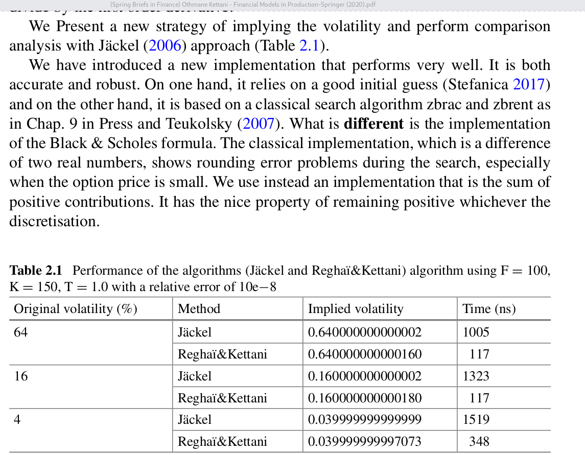
I stumbled upon a new short book Financial Models in Production from O. Kettani and A. Reghai. A page attracted my attention
A page from Kettani and Reghai's book.
This is the same example as I used on my blog, where I also present the Li’s SOR method combined with the good initial guess from Stefanica. The idea has also been expanded on in Jherek Healy’s book. What is shocking is that, beside reusing my example, they reuse my timing for Jäckel and my implementation is in Google Go, with a timing done on some older laptop. The numbers given are thus highly inconsistent. Of course, none of this is mentioned anywhere, and the book does not reference my blog.
I also find the description of how they improve the implied volatility algorithm (detailed on the next page) to not make much sense. After this kind of stuff, you can’t really trust anything that is in the book…
Worst perhaps, is that the authors advertise their “novel” technique in otherwise decent talks and conferences, such as the one from mathfinance. Here is a quote
Enforced Numerical Monotonicity (ENM) beats Jäckel’s implied volatility calculations – an implied vol calculator that never breaks and automatically fits vanilla option prices.
It is really unfortunate that the world we live in encourages such boasting. Papers always need to present some novel ideas to be published, but there is too often no check on whether the idea actually works, or is worth it. The temptation to make exagerated claims is very high for authors. In the end, it becomes not so easy to sort out the good from the bad.
I was wondering what were exactly the eigenvalues of the Mersenne-Twister random number generator transition matrix. An article by K. Savvidy sparked my interest on this.
This article mentioned a poor entropy (sum of log of eigenvalues amplitudes which are greater than 1), with eigenvalues falling almost on the unit circle.
The eigenvalues are also the roots of the characteristic polynomial. It turns out, that for jumping ahead in the random number sequence, we use the characteristic polynomial. There is a twist however,
we use it in F2 (modulo 2), for entropy, we are interested in the characteristic polynomial in Z (no modulo), specified in Appendix A of the Mersenne-Twister paper. The roots of the two polynomials are of course very different.
Now the degree of the polynomial is 19937, which is quite high. I searched for some techniques to compute quickly the roots, and found the paper “Efficient high degree polynomial root finding
using GPU”, whose main idea is relatively simple: use the Aberth method, with a Gauss-Seidel like iteration (instead of a Jacobi like iteration) for parallelization. Numerical issues are supposedly
handled by taking the log of the polynomial and its derivative in the formulae.
When I tried this, I immediately encountered numerical issues due to the limited precision of 64-bit floating point numbers. How to evaluate the log of the polynomial (and its derivative) in a stable way? It’s just not a simple problem at all.
Furthermore, the method is not particularly fast either compared to some other alternatives, such as calling eigvals on the companion matrix, a formulation which tends to help avoiding limited precision issues. And it requires a very good initial guess (in my case, on the unit circle, anything too large blows up).
The authors in the paper do not mention which polynomials they actually have tested, only the degree of some “full polynomial” and some “sparse polynomial”, and claim their technique works with full polynomials of degree 1 000 000 ! This may be true for some very specific polynomial where the log gives an accurate value, but is just plain false for the general case.
I find it a bit incredible that this gets published, although I am not too surprised since the bar for publication is low for many journals (see this enlightening post by J. Healy), and even for more serious journals, referees almost never actually try the method in question, so they have to blindly trust the results and focus mostly on style/presentation of ideas.
Fortunately, some papers are very good, such as Fast and backward stable computation of roots of polynomials, Part II: backward error analysis; companion matrix and companion pencil. In this case, the authors even provide a library in Julia, so the claims can be easily verified, and without surprise, it works very well, and is (very) fast. It also supports multiple precision, if needed. For the specific case of the Mersenne-Twister polynomial, it leads to the correct entropy value, working only with 64-bit floats, even though many eigenvalues have a not-so-small error. It is still relatively fast (compared to a standard LinearAlgebra.eigvals) using quadruple precision (128-bits), and there, the error in the eigenvalues is small.
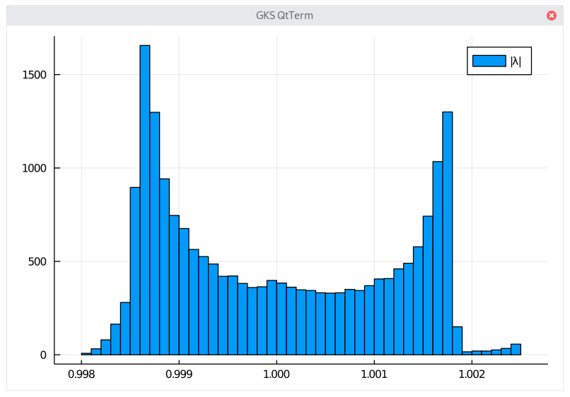
Overall, I found with this method an entropy of 10.377 (quite different from what is stated in K. Savvidy paper), although the plot of the distribution looks similar (but with a different scale: the total number of eigenvalues reported in K. Savvidy paper just does not add up to 19937, which is somewhat puzzling). A naive companion matrix solution led to 10.482. More problematic, if we look directly for the eigenvalues of the Mersenne-Twister transition matrix (Appendix A of the MT paper), we find 10.492, perhaps it is again an issue with the limited precision of 64-bits here.
Distribution of the eigenvalues of the Mersenne-Twister.
Below is the Mersenne-Twister polynomial, expressed in Julia code.
using DynamicPolynomials
import AMRVW
using Quadmath
@polyvar t
n =624m =397cp = DynamicPolynomials.Polynomial((t^n+t^m)*(t^(n-1)+t^(m-1))^31+(t^n+t^m)*(t^(n-1)+t^(m-1))^30+(t^n+t^m)*(t^(n-1)+t^(m-1))^29+(t^n+t^m)*(t^(n-1)+t^(m-1))^28+(t^n+t^m)*(t^(n-1)+t^(m-1))^27+(t^n+t^m)*(t^(n-1)+t^(m-1))^26+(t^n+t^m)*(t^(n-1)+t^(m-1))^24+(t^n+t^m)*(t^(n-1)+t^(m-1))^23+(t^n+t^m)*(t^(n-1)+t^(m-1))^18+(t^n+t^m)*(t^(n-1)+t^(m-1))^17+(t^n+t^m)*(t^(n-1)+t^(m-1))^15+(t^n+t^m)*(t^(n-1)+t^(m-1))^11+(t^n+t^m)*(t^(n-1)+t^(m-1))^6+(t^n+t^m)*(t^(n-1)+t^(m-1))^3+(t^n+t^m)*(t^(n-1)+t^(m-1))^2+1)
c = zeros(Float128,DynamicPolynomials.degree(terms(cp)[1])+1)
for te in terms(cp)
c[DynamicPolynomials.degree(te)+1] = coefficient(te)
endv128 = AMRVW.roots(c)
sum(x -> log(abs(x)),filter(x -> abs(x) >1, v128))
Several years ago, I read the book No Logo from Naomi Klein. I did not find it particularly good, but it did raise a valid concern overall.
This summer I read Shock Therapy - The rise of disaster capitalism. It suffers from some of the same flaws as No Logo, namely a lot of repetition of the same idea. Here, the underlying idea is that neoliberalism does not work in practice, and often ends up being some kind of corporatism. At the same time, it is suggested that some mild socialism is often much better for the people, although, the latter is not backed by concrete examples in the book. The former is backed by numerous documents, and is analyzed accross time and countries. It starts with Chili under Pinochet, the prototypical example that force is required to impose neoliberalism, then moves around South America in general, with some cases where a strong inflation, may be enough for the people to accept neoliberalism. Then it continues with China under Deng Xiao Ping, which I find a bit too much of a stretch to make a case about any kind of neoliberalism. Russia under Yeltsin is next, and it ends with the war in Irak and the USA.
The most interesting chapters are probably the first one, and the one about Irak. The first chapter explains the creation of the shock therapy treament by psychatrists and how it morphed to become a CIA “interrogation” technique. The chapter on Irak explains in details how people high up in the government reduced the public military staff/budget, and at the same time increased significantly the budget for contractors/external companies, which were closely linked to members of the government. It also makes you understand why it ended up being such a massive failure, even though it was presented as a Marshall plan for the middle east by the American government.
The worst chapters are definitely the introduction and the conclusion. The introduction is just not interesting, and the conclusion is saying that things are becoming better for the socialists, with the changes in South America (Chavez, Ecuador, Bolivia), all of which did not really stand the test of time, since the book was written.
Some annoying facts I found is that Milton Friedman is often made to be some sort of devil and Jeffrey Sachs is portrayed during the first half as his acolyte, and then he appears much more balanced when the author has an actual interview with him. The author however did not rewrite the previous chapters, so there is some sort of inconsistency there.
More annoying is that no positive aspect of neoliberalism ideas is presented, and socialism is often presented as a better alternative, without any proof. There are so many daily life examples that show where socialism is worse than liberalism. Recently, I had to contact a company for issues on my roof. The owner of this small company did not hesitate to say
“It is difficult to find people for this kind of job, because it is not always easy with the cold or the heat. People prefer to work at the city hall, where they are always three to do anything: one to carry the tools, one to watch, and one to actually do the work. In my company, we have to do everything alone”.
Another example that struck me recently is how bad are the school books. Although those are not written by the public workers, they need some sort of approval by those, and it ends up being a very small circle who can actually have those books accepted and distributed to schools. Only a few books are accepted and those will sell in the 10K+ quantity easily. In contrast, holiday children study books, which the parents are free to buy or not at any shop, are amazingly good. Indeed, if they were bad, almost nobody would buy them.
That being said, I don’t think liberalism is always good and socialism always bad either, there is probably a delicate balance somewhere.