The Gaussian kernel (as well as to some extent the smoothing spline) let us believe that there are multiple modes in the distribution (multiple peaks in the density). In reality,
Gaussian kernel approaches will, by construction, tend to exhibit such modes. It is not so obvious to know if those are real or artificial. There are other ways to apply the Gaussian kernel,
for example by optimizing the nodes locations and the standard deviation of each Gaussian. The resulting density with those is very similar looking.
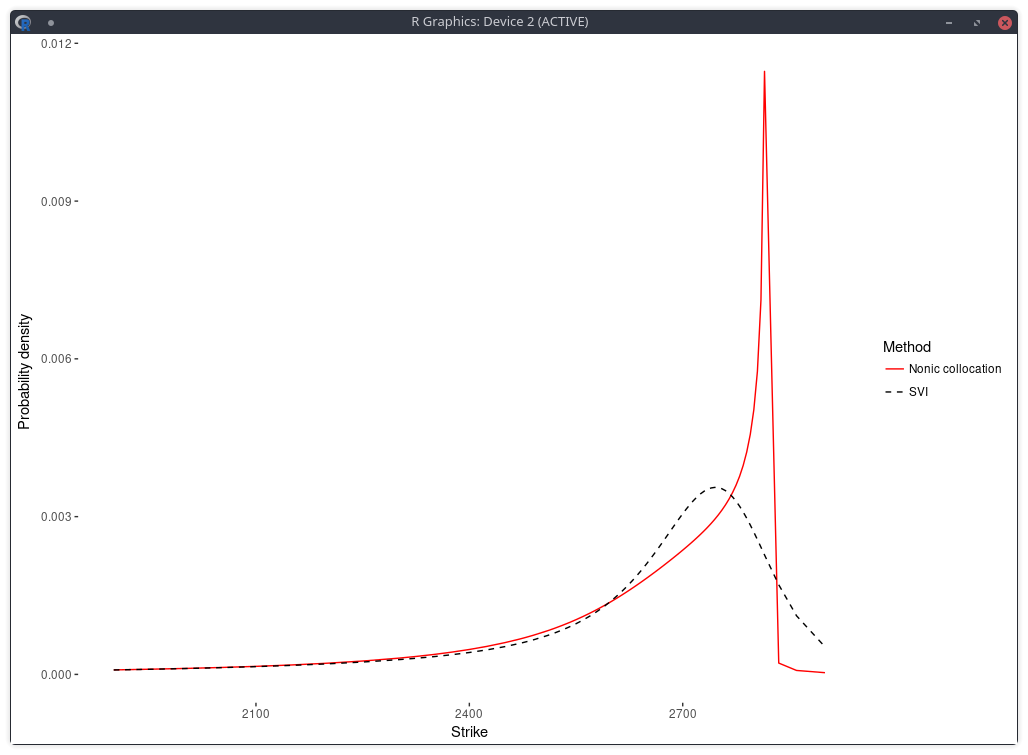
Following is the risk neutral density implied by nonic polynomial collocation out of the same quotes (Kees and I were looking at robust ways to apply the stochastic collocation):
probability density of the SPX implied from 1-month SPW options with stochastic collocation on a nonic polynomial.
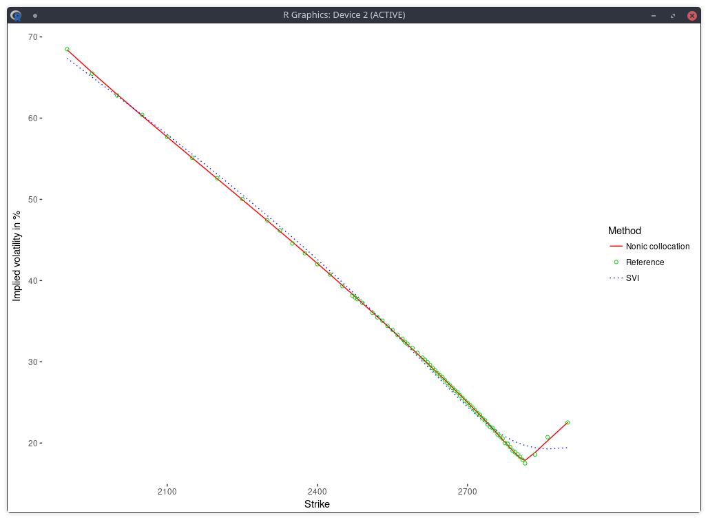
There is now just one mode, and the fit in implied volatilities is much better.
implied volatility of the SPX implied from 1-month SPW options with stochastic collocation on a nonic polynomial.
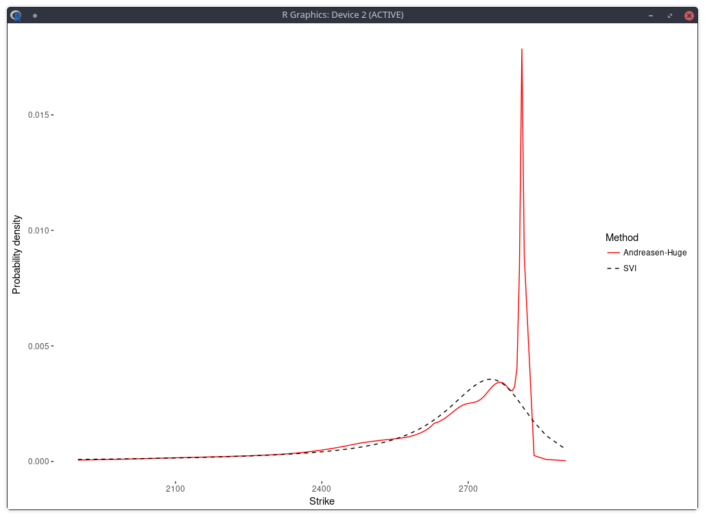
In a related experiment, Jherek Healy showed
that the Andreasen-Huge arbitrage-free single-step interpolation will lead to a noisy RND.
Sebastian Schlenkrich uses a simple regularization to calibrate his own piecewise-linear local volatility approximation
(a Lamperti-transform based approximation instead of the single step PDE approach of Andreasen-Huge).
His Tikhonov regularization consists here in applying a roughness penalty consisting
in the sum of squares of the consecutive local volatility slope differences. This is nearly the same as using the matrix of discrete second derivatives as Tikhonov matrix. The same idea can be found in cubic spline smoothing.
This roughness penalty can be added in the calibration of the Andreasen-Huge piecewise-linear discrete local volatilities and we obtain then a smooth RND:
density of the SPX implied from 1-month SPW options with Andreasen-Huge and Tikhonov regularization.
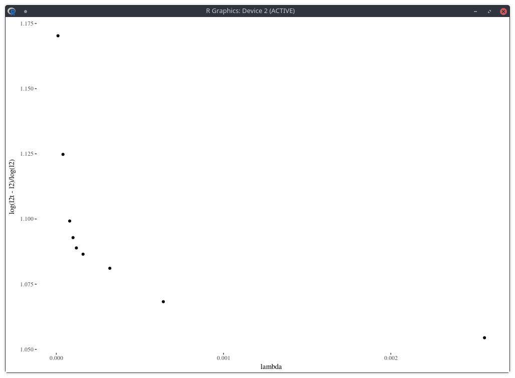
One difficulty however is to find the appropriate penalty factor \( \lambda \). On this example, the optimal penalty factor can be guessed from the L-curve which consists in plotting
the L2 norm of the objective against the L2 norm of the penalty term (without the factor lambda) in log-log scale, see for example this document. Below I plot a closely related function: the log of the penalty (with the lambda factor) divided by the log of the objective, against lambda. The point of highest curvature corresponds to the optimal penalty factor.
density of the SPX implied from 1-month SPW options with nodes located at every 2 market strike.
Note that in practice, this requires multiple calibrations the model with different values of the penalty factor, which can be slow.
Furthermore, from a risk perspective, it will also be challenging to deal with changes in the penalty factor.
The error of model versus market implied volatilies is similar to the nonic collocation (not better) even though the shape is less smooth and, a priori, less constrained as,
on this example, the Andreasen-Huge method has 75 free-parameters while the nonic collocation has 9.
It has been a while since the good old object-oriented (OO) programming is not trendy anymore. Functional programming or more dynamic programming (Python-based) have been the trend, with an excursion in template based programming for C++ guys. Those are not strict categories: Python can be used in a very OO way, but it’s not how it is marketed or considered by the community.
Recently, I have seen some of the ugliest refactoring in my life as a programmer, done by someone with at least 10 years of experience programming in Java. It is a good illustration because the piece of code is particularly simple (although I won’t bother with implementation details). The original code was a simple boolean method on an object such as
This is really breaking OO and moving back to procedural programming.
In a big (but not that big in reality) company, it is quite a challenge to avoid such code transformations. The code might be written by a team with a different manager, managers try to play nice to each other. And is it really worth fighting over such a trivial thing? if some low level (in the company hierarchy) programmer reports this, he is more likely to be labeled as a black sheep. Most managers prefer white sheeps.
More generally software is like entropy: it can start from a simple and clean state, but eventually it will always grow complex and somewhat ugly. And you end up with the Cobol syndrome, where people don’t really know anymore what the software is doing, can’t replace it as it is used (but nobody can tell exactly which parts), and “developers” do only small fixes and evolutions (patches) in an obsolete language on a system they don’t really understand.
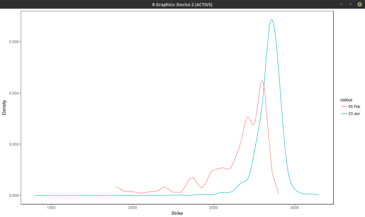
In the previous post, I showed a plot of the probability implied from SPW options before and after the big volatility change of last week.
I created it from a least squares spline fit of the market mid implied volatilities (weighted by the inverse of the bid-ask spread). While it looks reasonable, the underlying
technique is not very robust. It is particularly sensitive to the number of options strikes used as spline nodes.
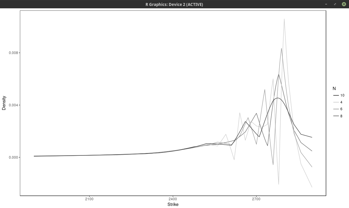
Below I vary the number of nodes, by considering nodes at every N market strikes, for different values of N.
probability density of the SPX implied from 1-month SPW options with nodes located at every N market strike, for different values of N. Least squares spline approach
With \(N \leq 6\), the density has large wiggles, that go into the negative half-plane. As expected, a large N produces a flatter and smoother density. It is not
obvious which value of N is the most appropriate.
Another technique is to fit directly a weighted sum of Gaussian densities, of fixed standard deviation, where the weights are calibrated to the market option prices. This is
described in various papers and books from Wystup such as this one. He calls it the kernel slice approach.
If we impose that the weights are positive and sum to one, the resulting model density will integrate to one and be positive.
It turns out that the price of a Vanilla option under this model is just the sum of vanilla options prices under the Bachelier model with shifted forwards (each “optionlet”
forward corresponds to a peak on the market strike axis). So it is easy and fast to compute. But more importantly, the problem of finding the weights is linear. In deed, the typical
measure to minimize is:
$$ \sum_{i=0}^{n} w_i^2 \left( C_i^M -\sum_{j=1}^m Q_j C_j^B(K_i) \right)^2 $$
where \( w_i \) is a market weight related to the bid-ask spread, \( C_i^M \) is the market option price with strike \( K_i \), \( C_j^B(K_i) \) is the j-th Bachelier
optionlet price with strike \( K_i \) and \( Q_j \) is the optionlet weight we want to optimize.
The minimum is located where the gradient is zero.
$$ \sum_{i=0}^{n} 2 w_i^2 C_k^B(K_i) \left( C_i^M -\sum_{j=1}^m Q_j C_j^B(K_i) \right) = 0 \text{ for } k=1,…,m $$
It is a linear and can be rewritten in term of matrices as \(A Q = B\) but we have the additional constraints
$$ Q_j \geq 0 $$
$$ \sum_j Q_j = 1 $$
The last constraint can be easily added with a Lagrange multiplier (or manually by elimination). The positivity constraint requires more work. As the problem is convex,
the solution must lie either inside or on a boundary. So we need to explore each case where \(Q_k = 0\) for one or several k in 1,…m.
In total we have \(2^{m-1}-1\) subsets to explore.
How to list all the subsets of \( \{1,…,m\} \)? It turns out it is very easy by using a bijection of each subset with the binary representation of \( {0,…,2^m} \). We then just need
to increment a counter for 1 to \( 2^m \) and transform the binary representation to our original set elements. Each element of the subset corresponds to a 1 in the binary representation.
Now this works well if m is not too large as we need to solve \(2^{m-1}-1\) linear systems.
I actually found amazing, it took only a few minutes for m as high as 26 without any particular optimization. For m larger we need to be more clever.
One possibility is to solve the unconstrained problem, and put all the negative quantities to 0 in the result, then solve again this new problem on those boundaries and repeat
until we find a solution. This simple algorithm works often well, but not always. There exists specialized algorithms that are much better and nearly as fast.
Unfortunately I was too lazy to code them. So I improvised on the Simplex. The problem can be transformed into something solvable by the Simplex algorithm.
We maximize the function \( -\sum_j Z_j \) with the constraints
$$ A Q - I Z = B $$
$$ Q_j \geq 0 $$
$$ Z_j \geq 0 $$
where I is the identity matrix. The additonal Z variables are slack variables, just here to help transform the problem. This is a trick I found on a researchgate forum. The two problems
are not fully equivalent, but they are close enough that the Simplex solution is quite good.
With the spline, we minimize directly bid-ask weighted volatilities. With the kernel slice approach, the problem is linear only terms of call prices. We could use a non-linear solver
with a good initial guess. Instead, I prefer to transform the weights so that the optimal solution on weighted prices is similar to the optimal solution on weighted volatilities.
For this, we can just compare the gradients of the two problems:
$$ \sum_{i=0}^{n} 2 {w}_i^2 \frac{\partial C}{\partial \xi}(\xi, K_i) \left( C_i^M - C(\xi, K_i) \right) $$
with
$$ \sum_{i=0}^{n} 2 {w^\sigma_i}^2\frac{\partial \sigma}{\partial \xi}(\xi, K_i) \left( \sigma_i^M - \sigma(\xi, K_i)\right) $$
As we know that
$$ \frac{\partial C}{\partial \xi} = \frac{\partial \sigma}{\partial \xi} \frac{\partial C}{\partial \sigma} $$
we approximate \( \frac{\partial C}{\partial \sigma} \) by the market Black-Scholes Vega and
\( \left( C_i^M - C(\xi, K_i) \right) \) by \( \frac{\partial C}{\partial \xi} (\xi_{opt}-\xi) \),
\( \left( \sigma_i^M - \sigma(\xi, K_i) \right) \) by \( \frac{\partial \sigma}{\partial \xi} (\xi_{opt}-\xi) \)
to obtain
$$ {w}_i \approx \frac{1}{ \frac{\partial C_i^M}{\partial \sigma_i^M} } {w^\sigma_i} $$
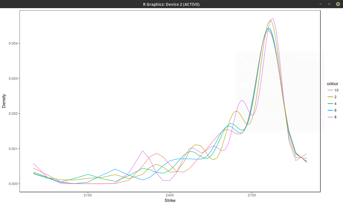
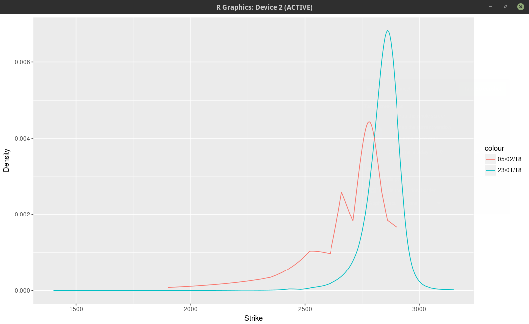
Now it turns out that the kernel slice approach is quite sensitive to the choice of nodes (strikes), but not as much as to the choice of number of nodes. Below is
the same plot as with the spline approach, that is we choose every N market strike as node. For N=4, the density is composed of the sum of m/4 Gaussian densities. We
optimized the kernel bandwidth (here the standard deviation of each Gaussian density), and found that it was relatively insensitive to the number of nodes,
in our case around 33.0 (in general it is expected to be about three times the order the distance between two consecutive strikes, which is 5 to 10 in our case), a smaller value will translate to
narrower peaks.
probability density of the SPX implied from 1-month SPW options with nodes located at every N market strike, for different values of N. Kernel slice approach.
Even if we consider here more than 37 nodes (m=75 market strikes), the optimal solution actually use only 13 nodes, as all the other nodes have a calibrated weight of 0.
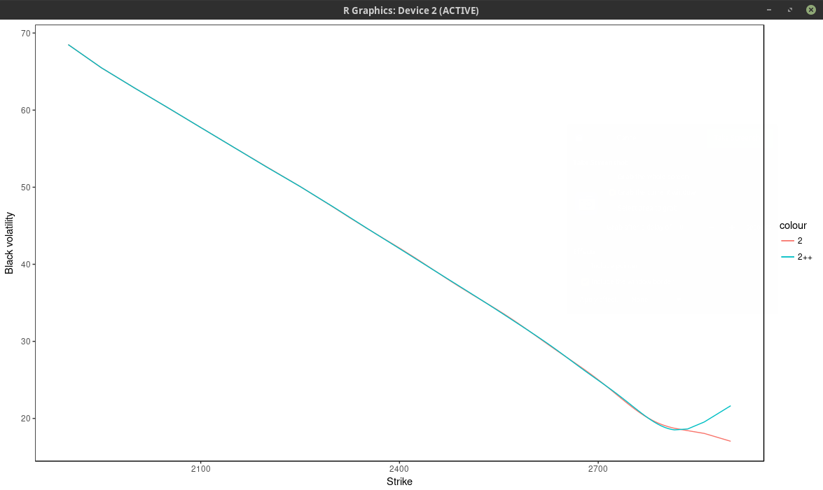
The fit can be much better by adding nodes at
f * 0.5, f * 0.8, f * 0.85, f * 0.9, f * 0.95, f * 0.98, f, f * 1.02, f * 1.05, f * 1.1, f * 1.2, f * 1.5, where f is the forward price, even though the optimal solution
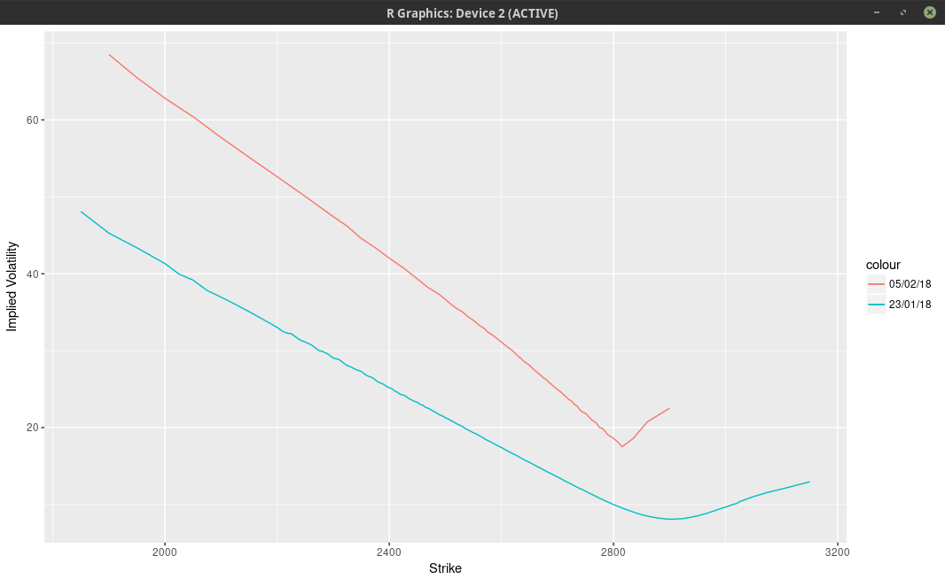
will only use 13 nodes again. We can see this by looking at the implied volatility.
implied volatility of the SPX implied from 1-month SPW options with nodes located at every 2 market strike.
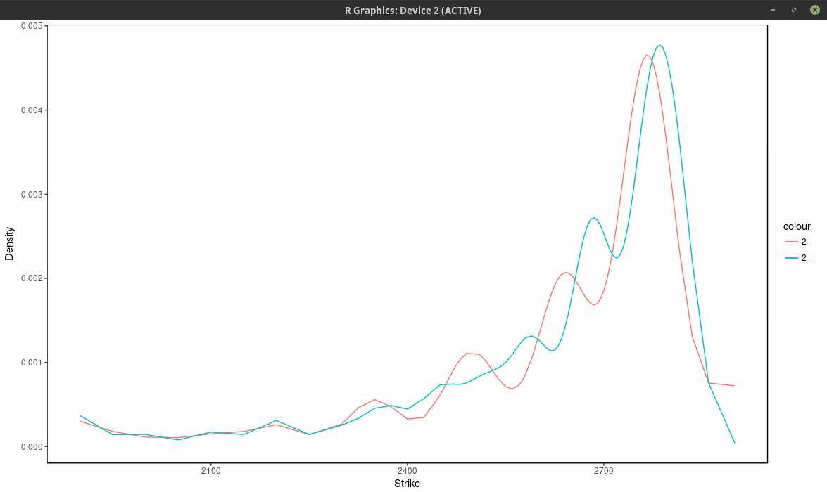
Using only the market nodes does not allow to capture right wing of the smile. The density is quite different between the two.
density of the SPX implied from 1-month SPW options with nodes located at every 2 market strike.
I found (surprisingly) that even those specific nodes by themselves (without any market strike) work better than using all market strikes (without those nodes), but
then we impose where the peaks will be located eventually.
It is interesting to compare the graph with the one before the volatility jump:
density of the SPX implied from 1-month SPW options with nodes located at every 2 market strike.
So in calm markets, the density is much smoother and has really only one main mode/peak.
It is possible to use other kernels than the Gaussian kernel. The problem to solve would be exactly the same. It is not clear what would be the advantages
of another kernel, except, possibly, speed to solve the linear system in O(n) operations for a compact kernel spanning at most 3 nodes (which would translate to a tridiagonal system).
Yesterday the American stocks went a bit crazy along with the VIX that jumped from 17.50 to 38. It’s not exactly clear why, the news mention that the Fed might raise its interest rates, the bonds yield have been recently increasing substantially, and the market self-correcting
after stocks grew steadily for months in a low VIX environment.
I don’t exactly follow the SPX/SPW options daily. But I had taken a snapshot two weeks ago when the market was quiet. We can imply the probability density from the market option prices.
It’s not an exact science. Here I do this with a least-squares spline on the implied volatilities (the least squares smoothes out the noise). I will show another approach in a subsequent post.
probability density of the SPX implied from 1-month SPW options.
We can clearly see two bumps and a smaller third one further away in the left tail. This means that the market participants expect the SPX500 to go mostly to 2780 (slightly below where the spx future used to be) one month from now.
Some market participants are more cautious and believe it could hover around 2660. Finally a few pessimists think more of 2530.
Option traders like to look at the implied volatilities (below).
implied volatilities of 1-month SPW options.
On the graph above, it’s really not clear that there is some sort of trimodal distribution. There is however an extremely sharp edge, that we normally see only for much shorter maturities. The vols are interpolated with
a cubic spline above, not with a least-squares spline, in order to show the edge more clearly.
Several months ago, I had a quick look at a recent paper describing how to use
Wavelets to price options under stochastic volatility models with a known characteristic function.
The more classic method is to use some numerical quadrature directly on the Fourier integral as described in this paper for example.
When I read the paper, I was skeptical about the Wavelet approach, since it looked complicated, and with many additional parameters.
I recently took a closer look and it turns out my judgment was bad. The additional parameters can be easily automatically and reliably set
by very simple rules that work well (a subsequent paper by the same author, which applies the method to Bermudan options, clarifies this).
The method is also not as complex as I first imagined. And more importantly, the FFT makes it fast. It is quite amazing to see
the power of the FFT in action. It really is because of the FFT that the Shannon Wavelet method is practical.
Anyway one of the things that need to be computed are the payoff coefficients, and one expression is just the sum of a discrete Cosine transform (DCT) and a discrete Sine transform (DST).
I was wondering then
about a simple way to use the FFT for the Sine transform. There are many papers around how to use the FFT to compute the Cosine transform. A technique
that is efficient and simple is the one of Makhoul.
The coefficients that need to be computed for all k can be represented by the following equation
$$ V_{k} = \sum_{j=0}^{N-1} a_j \cos\left(\pi k\frac{j+\frac{1}{2}}{N}\right) + b_j \sin\left(\pi k\frac{j+\frac{1}{2}}{N}\right) $$
with \( N= 2^{\bar{J}-1} \) for some positive integer \( \bar{J} \).
Makhoul algorithm to compute the DCT of size N with one FFT of size N consists in
and then from the result of the FFT \( hat{c} \), the DCT coefficients \( \hat{a} \) are
$$ \hat{a}_k = \Re\left[ \hat{c}_j e^{-i \pi\frac{k}{2N}} \right],. $$
Makhoul does not specify the equivalent formula for the DST, but we can do something similar.
We first initialize the FFT coefficients \( c_j \) with:
$$ c_j = b_{2j} \quad,,\quad c_{N-1-j} = -b_{2j+1} \quad \text{ for } j = 0,…, \frac{N}{2}-1 $$
and then from the result of the FFT \(\hat{c}\), the DST coefficients \(\hat{b}\) are
$$\hat{b}_k = -\Im\left[ \hat{c}_j e^{-i \pi\frac{k}{2N}} \right],. $$
For maximum performance, the two FFTs can reuse the same sine and cosine tables. And the last step of the DCT and DST can be combined together.
Another approach would be to compute a single FFT of size 2N as we can rewrite the coefficients as
$$ V_{k} = \Re\left[e^{-i \pi \frac{k}{2N}} \sum_{j=0}^{2N-1} (a_j + i b_j) e^{-2i\pi k\frac{j}{2N}} \right] $$
with \(a_j = b_j =0 \) for \( j \geq N \)
In fact the two are almost equivalent, since a FFT of size 2N is decomposed internally into two FFTs of size N.
With this in mind we can improve a bit the above to merge the two transforms together:
We first initialize the FFT coefficients \( c_j \) with:
$$ c_j = a_{2j} + i b_{2j} \quad,,\quad c_{N-1-j} = a_{2j+1} -i b_{2j+1} \quad \text{ for } j = 0,…, \frac{N}{2}-1 $$
and then from the result of the FFT \(\hat{c}\), the coefficients are
$$V_k = \Re\left[ \hat{c}_j e^{-i \pi\frac{k}{2N}} \right],. $$
And we have computed the coefficients with a single FFT of size N.
In terms of Go language code, the classic type-2 sine Fourier transforms reads
funcDST2(vector []float64) error {
n :=len(vector)
result :=make([]float64, n)
for k :=range vector {
sum :=0.0for j, vj :=range vector {
sum += math.Sin((float64(j)+0.5)*math.Pi*float64(k)/float64(n)) * vj
}
result[k] = sum
}
copy(vector, result)
returnnil}
And the Fast Type-2 Sine transform reads
funcFastDST2ByFFT(vector []float64) error {
n :=len(vector)
halfLen := n /2 z :=make([]complex128, n)
for i :=0; i < halfLen; i++ {
z[i] = complex(vector[i*2], 0)
z[n-1-i] = complex(-vector[i*2+1], 0)
}
if n&1==1 {
z[halfLen] = complex(vector[n-1], 0)
}
err :=TransformRadix2Complex(z)
for i :=range z {
temp :=float64(i) * math.Pi /float64(n*2)
s, c := math.Sincos(temp)
vector[i] = real(z[i])*s -imag(z[i])*c
}
return err
}
The function TransformRadix2Complex, used above, steams from a standard implementation of the discrete Fourier transform (DFT) of the given complex vector, storing the result back into the vector (The vector’s length must be a power of 2. Uses the Cooley-Tukey decimation-in-time radix-2 algorithm).
funcTransformRadix2Complex(z []complex128) error {
n :=len(z)
levels :=uint(31- bits.LeadingZeros32(uint32(n))) // Equal to floor(log2(n))
if (1<< levels) != n {
return fmt.Errorf("Length is not a power of 2")
}
// Trigonometric tables
cosTable, sinTable :=MakeCosSinTable(n)
// Bit-reversed addressing permutation
for i :=range z {
j :=int(bits.Reverse32(uint32(i)) >> (32- levels))
if j > i {
z[i], z[j] = z[j], z[i]
}
}
// Cooley-Tukey decimation-in-time radix-2 FFT
for size :=2; size <= n; size *=2 {
halfsize := size /2 tablestep := n / size
for i :=0; i < n; i += size {
j := i
k :=0for ; j < i+halfsize; j++ {
l := j + halfsize
tpre :=real(z[l])*cosTable[k] +imag(z[l])*sinTable[k]
tpim :=-real(z[l])*sinTable[k] +imag(z[l])*cosTable[k]
z[l] = z[j] -complex(tpre, tpim)
z[j] +=complex(tpre, tpim)
k += tablestep
}
}
if size == n { // Prevent overflow in 'size *= 2'
break }
}
returnnil}
funcMakeCosSinTable(n int) ([]float64, []float64) {
cosTable :=make([]float64, n/2)
sinTable :=make([]float64, n/2)
for i :=range cosTable {
s, c := math.Sincos(2* math.Pi *float64(i) /float64(n))
cosTable[i] = c
sinTable[i] = s
}
return cosTable, sinTable
}
Interest Rate Derivatives Explained: Volume 1: Products and Markets by Jörg Kienitz. It refers to my paper on curve interpolation (there is a mistake in the actual reference given inside the book,about arbitrage-free SABR, which unrelated to the text). I like how this book gives real world market data related to the products considered.
It is a relatively common belief that the vanilla Android experience is better, as it runs smoother. The Samsung Touchwiz is often blamed for making things slow and not more practical.
I have had a Nexus 6 for a couple of years and I noticed the slowdowns after each update, up to a point where it sometimes took a few seconds to open the phone app, or to display the keyboard. I freed up storage, removed some apps but this did not make any difference. This is more or less the same experience that people have with the Samsung devices if reddit comments are to be believed.
The other myth is that Google phones will be updated for a longer time. Prior to the Nexus 6, I had a Galaxy Nexus, which Google stopped supporting after less than 2 years. The Nexus 6 received security update until this October, that is nearly 2 years for me and 2.5 years for early buyers.
In comparison Apple updates its phones for much longer and a 4 years old iphone 5s still runs smoothly. Fortunately for Android phones, there are the alternative roms. Being desperate with the state of my Nexus phone, I installed paranoid android. I am surprised at how good it is. My phone feels like new again, and as good as any flagship I would purchase today. To my great surprise I did not find any clear step by step installation process for Paranoid Android. I just followed the detailed steps for LineageOS (CyanogenMod descendent), but with the paranoid android zip file instead of the LineageOS one. I have some trouble to understand how some open source ROM can be much nicer than the pure Google Android ROM, but it is. I have had no crash/reboot (which became more common as well with the years), plus it’s still updated regularly. Google does not set a good standard by not supporting its own devices better.
There is however one thing that Google does well, it’s the camera app. The HDR+ mode makes my Nexus 6 take great pictures, even compared to new android phones or iphones. I am often amazed at the pictures I manage to take, and others are also amazed at how good they look (especially since they look often better on the Nexus 6 screen than on a computer monitor). Initially I remember the camera to be not so great, but some update that came in 2016 transformed the phone into a fantastic shooter. It allowed me to take very nice pictures in difficult conditions, see for example this google photo gallery. Fortunately it’s still possible to install the app in the Google Play store on Paranoid Android. They should really make it open-source and easier to adapt it to other android phones.
A photo made with the Google camera app on the Nexus 6.
A few years ago, when Git was rising fast and SVN was already not hype anymore, a friend thought that SVN was for many organizations better suited than Git, with the following classical arguments, which were sound at the time:
Who needs decentralization for a small team or a small company working together?
SVN is proven, works well and is simple to use and put in place.
Each argument is in reality not so strong. It becomes clear now that Git is much more established.
Regarding the first argument, a long time ago some people had trouble with CVS as it introduced the idea of merging instead of locking files. Git represents a similar paradigm shift between the centralized and the decentralized. It can scare people in not so rational ways. You could lock files with CVS as you did with visual sourcesafe or any other crappy old source control system. It’s just that people favored merges as it was effectively more convenient and more productive. You can also use Git with a centralized workflow. Another more scary paradigm shift with Git is to move away from the idea that branches are separate folders. With Git you just switch branches as it is instantaneous even though, again, you could use it in the old fashioned SVN way.
Now onto the second argument, SVN is proven to work well. But so is Cobol. Today it should be clear that SVN is essentially dead. Most big projects move or have moved to git. Tools work better with Git, even Eclipse works natively with Git but requires buggy plugins for SVN. New developers don’t know SVN.
I heard other much worse arguments against Git since. For example, some people believed that, with Git, they could lose some of their code changes. This was partially due to sensational news article such as the Gitlab.com data loss, where in reality some administrator deleted some directory and had non-working backups. As a result, some Git repositories were deleted, but in reality it’s a common data loss situation, unrelated to the use of Git as version control system. This Stackoverflow question gives a nice overview of data loss risks with Git.
What I feel is true however is that Git is more complex than SVN, because it is more powerful and more flexible. But if you adopt a simple workflow, it’s not necessarily more complicated.
Machine learning and artificial intelligence are the current hype (again). In their new Ryzen processors, AMD advertises the Neural Net Prediction. It turns out this is was already used in their older (2012) Piledriver architecture used for example in the AMD A10-4600M. It is also present in recent Samsung processors such as the one powering the Galaxy S7. What is it really?
The basic idea can be traced to a paper from Daniel Jimenez and Calvin Lin “Dynamic Branch Prediction with Perceptrons”, more precisely described in the subsequent paper “Neural methods for dynamic branch prediction”. Branches typically occur in if-then-else statements. Branch prediction consists in guessing which code branch, the then or the else, the code will execute, thus allowing to precompute the branch in parallel for faster evaluation.
Jimenez and Lin rely on a simple single-layer perceptron neural network whose input are the branch outcome (global or hybrid local and global) histories and the output predicts which branch will be taken. In reality, because there is a single layer, the output y is simply a weighted average of the input (x, and the constant 1):
$$ y = w_0 + \sum_{i=1}^n x_i w_i $$
\( x_i = \pm 1 \) for a taken or not taken. \( y > 0 \) predicts to take the branch.
Ideally, each static branch is allocated its own perceptron. In practice, a hash of the branch address is used.
The training consists in updating each weight according to the actual branch outcome t : \( w_i = w_i + 1 \) if \( x_i = t \) otherwise \( w_i = w_i - 1 \). But this is done only if the predicted outcome is lower than the training (stopping) threshold or if the branch was mispredicted. The threshold keeps from overtraining and allow to adapt quickly to changing behavior.
The perceptron is one of those algorithms created by a psychologist. In this case, the culprit is Frank Rosenblatt. Another more recent algorithm created by a psychologist is the particle swarm optimization from James Kennedy. As in the case of particle swarm optimization, there is not a single well defined perceptron, but many variations around some key principles. A reference seems to be the perceptron from H.D. Block, probably because he describes the perceptron in terms closer to code, while Rosenblatt was really describing a perceptron machine.
The perceptron from H.D. Block is slightly more general than the perceptron used for branch prediction:
the output can be -1, 0 or 1. The output is zero if the weighted average is below a threshold (a different constant from the training threshold of the branch prediction perceptron).
reinforcement is not done on inactive connections, that is for \( x_i = 0 \).
a learning rate \( \alpha \) is used to update the weight: \( w_i += \alpha t x_i \)
The perceptron used for branch prediction is quite different from the deep learning neural networks fad, which have many more layers, with some feedback loop. The challenge of those is the training: when many layers are added to the perceptron, the gradients of each layer activation function multiply in the backpropagation algorithm. This makes the “effective” gradient at the first layers to be very small, which translates to tiny changes in the weights, making training not only very slow but also likely stuck in a sub-optimal local minimum. Beside the vanishing gradient problem, there is also the catastrophic interference problem to pay attention to. Those issues are today dealt with the use of specific strategies to train / structure the network combined with raw computational power that was unavailable in the 90s.
Around 15 years ago, I wrote a small Java applet to try and show the Benham disk effect. Even back then applets were already passé and Flash would have been more appropriate. These days, no browser support Java applets anymore, and very few web users have Java installed. Flash also mostly disappeared. The web canvas is today’s standard allowing to embbed animations in a web page.
This effect shows color perception from a succession of black and white pictures. It is a computer reproduction from the Benham disc with ideas borrowed from "Pour La Science Avril/Juin 2003".
Using a delay between 40 and 60ms, the inner circle should appear red, the one in the middle
blue and the outer one green. When you reverse the rotation direction,
blue and red circles should be inverted.