Bad papers and the roots of high degree polynomials
I was wondering what were exactly the eigenvalues of the Mersenne-Twister random number generator transition matrix. An article by K. Savvidy sparked my interest on this. This article mentioned a poor entropy (sum of log of eigenvalues amplitudes which are greater than 1), with eigenvalues falling almost on the unit circle.
The eigenvalues are also the roots of the characteristic polynomial. It turns out, that for jumping ahead in the random number sequence, we use the characteristic polynomial. There is a twist however, we use it in F2 (modulo 2), for entropy, we are interested in the characteristic polynomial in Z (no modulo), specified in Appendix A of the Mersenne-Twister paper. The roots of the two polynomials are of course very different.
Now the degree of the polynomial is 19937, which is quite high. I searched for some techniques to compute quickly the roots, and found the paper “Efficient high degree polynomial root finding using GPU”, whose main idea is relatively simple: use the Aberth method, with a Gauss-Seidel like iteration (instead of a Jacobi like iteration) for parallelization. Numerical issues are supposedly handled by taking the log of the polynomial and its derivative in the formulae.
When I tried this, I immediately encountered numerical issues due to the limited precision of 64-bit floating point numbers. How to evaluate the log of the polynomial (and its derivative) in a stable way? It’s just not a simple problem at all. Furthermore, the method is not particularly fast either compared to some other alternatives, such as calling eigvals on the companion matrix, a formulation which tends to help avoiding limited precision issues. And it requires a very good initial guess (in my case, on the unit circle, anything too large blows up).
The authors in the paper do not mention which polynomials they actually have tested, only the degree of some “full polynomial” and some “sparse polynomial”, and claim their technique works with full polynomials of degree 1 000 000 ! This may be true for some very specific polynomial where the log gives an accurate value, but is just plain false for the general case.
I find it a bit incredible that this gets published, although I am not too surprised since the bar for publication is low for many journals (see this enlightening post by J. Healy), and even for more serious journals, referees almost never actually try the method in question, so they have to blindly trust the results and focus mostly on style/presentation of ideas.
Fortunately, some papers are very good, such as Fast and backward stable computation of roots of polynomials, Part II: backward error analysis; companion matrix and companion pencil. In this case, the authors even provide a library in Julia, so the claims can be easily verified, and without surprise, it works very well, and is (very) fast. It also supports multiple precision, if needed. For the specific case of the Mersenne-Twister polynomial, it leads to the correct entropy value, working only with 64-bit floats, even though many eigenvalues have a not-so-small error. It is still relatively fast (compared to a standard LinearAlgebra.eigvals) using quadruple precision (128-bits), and there, the error in the eigenvalues is small.
Overall, I found with this method an entropy of 10.377 (quite different from what is stated in K. Savvidy paper), although the plot of the distribution looks similar (but with a different scale: the total number of eigenvalues reported in K. Savvidy paper just does not add up to 19937, which is somewhat puzzling). A naive companion matrix solution led to 10.482. More problematic, if we look directly for the eigenvalues of the Mersenne-Twister transition matrix (Appendix A of the MT paper), we find 10.492, perhaps it is again an issue with the limited precision of 64-bits here.
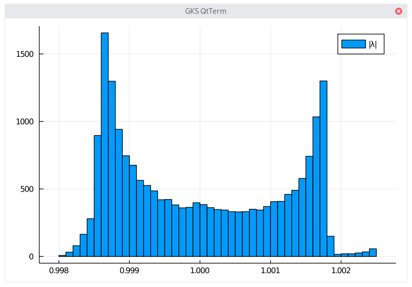
Distribution of the eigenvalues of the Mersenne-Twister.
Below is the Mersenne-Twister polynomial, expressed in Julia code.
using DynamicPolynomials
import AMRVW
using Quadmath

@polyvar t
n = 624
m = 397
cp = DynamicPolynomials.Polynomial((t^n+t^m)*(t^(n-1)+t^(m-1))^31+(t^n+t^m)*(t^(n-1)+t^(m-1))^30+(t^n+t^m)*(t^(n-1)+t^(m-1))^29+(t^n+t^m)*(t^(n-1)+t^(m-1))^28+(t^n+t^m)*(t^(n-1)+t^(m-1))^27+(t^n+t^m)*(t^(n-1)+t^(m-1))^26+(t^n+t^m)*(t^(n-1)+t^(m-1))^24+(t^n+t^m)*(t^(n-1)+t^(m-1))^23+(t^n+t^m)*(t^(n-1)+t^(m-1))^18+(t^n+t^m)*(t^(n-1)+t^(m-1))^17+(t^n+t^m)*(t^(n-1)+t^(m-1))^15+(t^n+t^m)*(t^(n-1)+t^(m-1))^11+(t^n+t^m)*(t^(n-1)+t^(m-1))^6+(t^n+t^m)*(t^(n-1)+t^(m-1))^3+(t^n+t^m)*(t^(n-1)+t^(m-1))^2+1)

c = zeros(Float128,DynamicPolynomials.degree(terms(cp)[1])+1)
for te in terms(cp)
  c[DynamicPolynomials.degree(te)+1] = coefficient(te)
end
v128 = AMRVW.roots(c)
sum(x -> log(abs(x)),filter(x -> abs(x) > 1, v128))