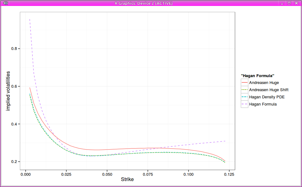
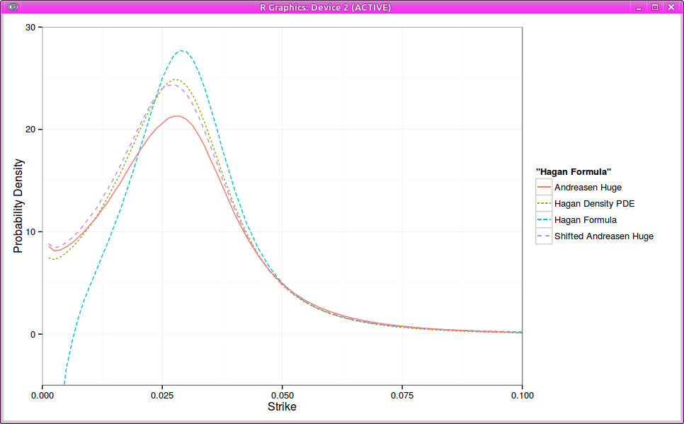
I looked nearly two years ago already at the arbitrage free SABR of Andreasen-Huge in comparison to the arbitrage free PDE of Hagan and showed how close the ideas were: Andreasen-Huge relies on the normal Dupire forward PDE using a slightly simpler local vol (no time dependent exponential term) while Hagan works directly on the Fokker-Planck PDE (you can think of it as the Dupire Forward PDE for the density) and uses an expansion of same order as the original SABR formula (which leads to an additional exponential term in the local volatility).
One clever idea from Andreasen-Huge is the use of a single step. It turns out that their idea is not completely new. Daniel Duffy sent me some old papers from Shishkin around fitted schemes (here is one). This is very much the same thing, except Shishkin concern is about a good handling of discontinuity in the initial condition, and therefore makes the association step function => cumulative density to fit the diffusion parameter. Andreasen-Huge work directly with the call prices as this is what they solve.
One drawback of Andreasen-Huge one step method is the inability to match the standard SABR smile: the parameters don’t have exactly the same meaning. It turns out that by just shifting proportionally the local volatility by a constant factor, Andreasen Huge matches Hagan PDE vols quite closely.
Implied Black volatilities
Probability density
While this is interesting in itself, it’s still not so simple to backup this factor without solving for it (and then the method looses appeal).
A few recent programming languages sparked my interest:
Julia because of the wide coverage of mathematical functions, and great attention to quality of the implementations. It has also some interesting web interface.
Dart: because it’s a language focused purely on building apps for the web, and has a supposedly good VM.
Rust: it’s the latest fad. It has interesting concepts around concurrency and a focus on being low level all the while being simpler than C.
I decided to see how well suited they would be on a simple Monte-Carlo simulation of a forward start option under the Black model. I am no expert at all in any of the languages, so this is a beginner’s test. I compared the runtime for executing 16K simulations times a multiplier.
Multipl.
Scala
Julia
JuliaA
Dart
Python
Rust
1
0.03
0.08
0.09
0.03
0.4
0.004
10
0.07
0.02
0.06
0.11
3.9
0.04
100
0.51
0.21
0.40
0.88
0.23
1000
4.11
2.07
4.17
8.04
2.01
About performance
I am quite impressed at Dart performance versus Scala (or vs. Java, as it has the same performance as Scala) given that it is much less strict about types and its focus is not at all on this kind of stuff.
Julia performance is great, that is if one is careful about types. Julia is very finicky about casting and optimizations, fortunately @time helps spotting the issues (often an inefficient cast will lead to copy and thus high allocation). JuliaA is my first attempt, with an implicit badly performing conversion of MersenneTwister to AbstractRNG. It is slower first, as the JIT costs is reflected on the first run, very much like in Java (although it appears to be even worse).
Rust is the most impressive. I had to add the –release flag to the cargo build tool to produce a properly optimized binary, otherwise the performance is up to 7x worse.<
About the languages
My Python code is not vectorized, just like any of the other implementations. While the code looks relatively clean, I made the most errors compared to Julia or Scala. Python numpy isn’t always great: norm.ppf is very slow, slower than my hand coded python implementation of AS241.
Dart does not have fixed arrays: everything is a list. It also does not have strict 64 bit int: they can be arbitrarily large. The dev environment is ok but not great.
Julia is a bit funny, not very OO (no object method) but more functional, although many OO concepts are there (type inheritence, type constructors). It was relatively straightforward, although I do not find intuitive the type conversion issues (eventual copy on conversion).
Rust took me the most time to write, as it has quite new concepts around mutable variables, and “pointers” scope. I relied on an existing MersenneTwister64 that worked with latest Rust. It was a bit disappointing to see that some dSFMT git project did not compile with the latest Rust, likely because Rust is still a bit too young. This does not sound so positive, but I found it to be the language the most interesting to learn.
I was familiar with Scala before this exercise. I used a non functional approach, with while loops in order to make sure I had maximum performance. This is something I find a bit annoying in Scala, I always wonder if for performance I need to do a while instead of a for, when the classic for makes much more sense (that and the fact that the classic for leads to some annoying delegation in runtime errors/on debug).
I relied on the default RNG for Dart but MersenneTwister for Scala, Julia, Python, Rust. All implementations use a hand coded AS241 for the inverse cumulative normal.
Update
Using FastMath.exp instead of Math.exp leads a slightly better performance for Scala:
Multipl.
Scala
1
0.06
10
0.05
100
0.39
1000
2.66
I did not expect that this would still be true in 2015 with Java 8 Oracle JVM.
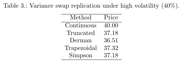
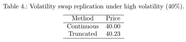
I have looked at jump effects on volatility vs. variance swaps. There is a similar behavior on tail events, that is, on truncating the replication. One main problem with discrete replication of variance swaps is the implicit domain truncation, mainly because the variance swap equivalent log payoff is far from being linear in the wings. The equivalent payoff with Carr-Lee for a volatility swap is much more linear in the wings (not so far of a straddle). So we could expect the replication to be less sensitive to the wings truncation.
I have done a simple test on flat 40% volatility:
As expected, the vol swap is much less sensitive, and interestingly, very much like for the jumps, it moves in the opposite direction: the truncated price is higher than the non truncated price.
Antonov et al. present an interesting view on SABR with negative rates: instead of relying on a shifted SABR to allow negative rates up to a somewhat arbitrary shift, they modify slightly the SABR model to allow negative rates directly:
$$ dF_t = |F_t|^\beta v_t dW_F $$
with \\( v\_t \\) being the standard lognormal volatility process of SABR.
Furthermore they derive a clever semi-analytical approximation for this model, based on low correlation, quite close to the Monte-Carlo prices in their tests. It's however not clear if it is arbitrage-free.
It turns out that it is easy to tweak Hagan SABR PDE approach to this "absolute SABR" model: one just needs to push the boundary \\(F\_{min}\\) far away, and to use the absolute value in C(F).
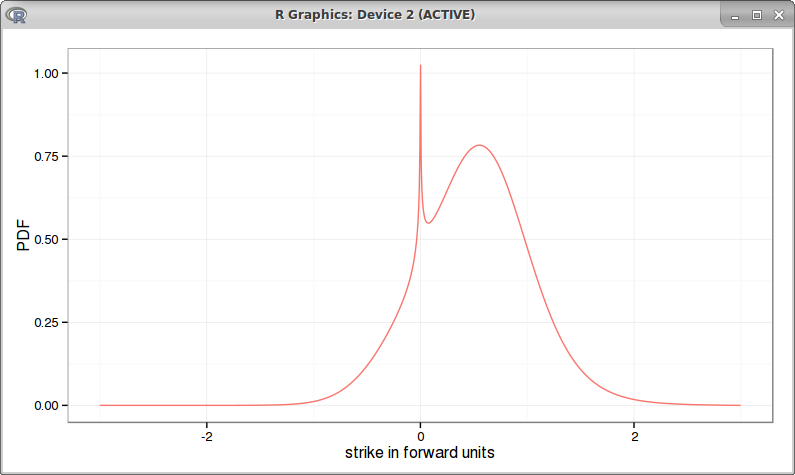
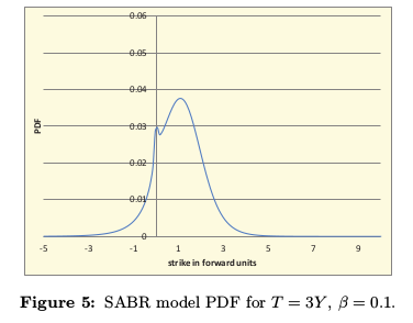
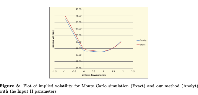
It then reproduces the same behavior as in Antonov et al. paper:
"Absolute SABR" arbitrage free PDE
Antonov et al. graph
I obtain a higher spike, it would look much more like Antonov graph had I used a lower resolution to compute the density: the spike would be smoothed out.
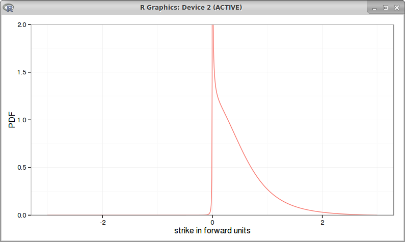
Interestingly, the arbitrage free PDE will also work for high beta (larger than 0.5):
beta = 0.75
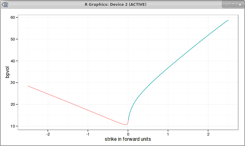
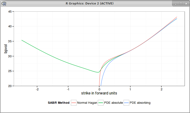
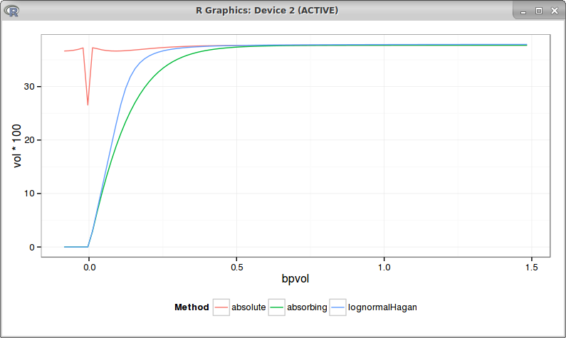
It turns out to be then nearly the same as the absorbing SABR, even if prices can cross a little the 0. This is how the bpvols look like with beta = 0.75:
red = absolute SABR, blue = absorbing SABR with beta=0.75
They overlap when the strike is positive.
If we go back to Antonov et al. first example, the bpvols look a bit funny (very symmetric) with beta=0.1:
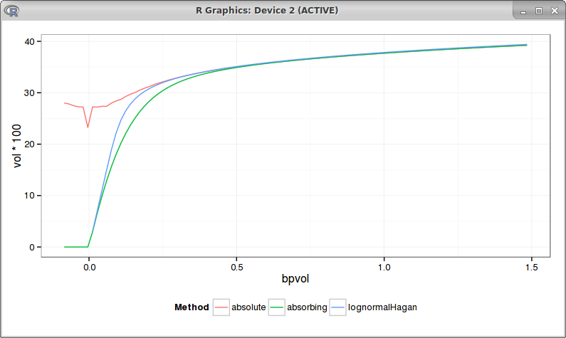
For beta=0.25 we also reproduce Antonov bpvol graph, but with a lower slope for the left wing:
bpvols with beta = 0.25
It's interesting to see that in this case, the positive strikes bp vols are closer to the normal Hagan analytic approximation (which is not arbitrage free) than to the absorbing PDE solution.
For longer maturities, the results start to be a bit different from Antonov, as Hagan PDE relies on a order 2 approximation only:
absolute SABR PDE with 10y maturity
The right wing is quite similar, except when it goes towards 0, it's not as flat, the left wing is much lower.
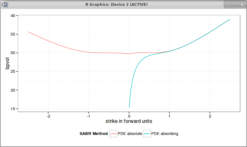
Another important aspect is to reproduce Hagan's knee, the atm vols should produce a knee like curve, as different studies show (see for example this recent Hull & White study or this other recent analysis by DeGuillaume). Using the same parameters as Hagan (beta=0, rho=0) leads to a nearly flat bpvol: no knee for the absolute SABR, curiously there is a bump at zero, possibly due to numerical difficulty with the spike in the density:
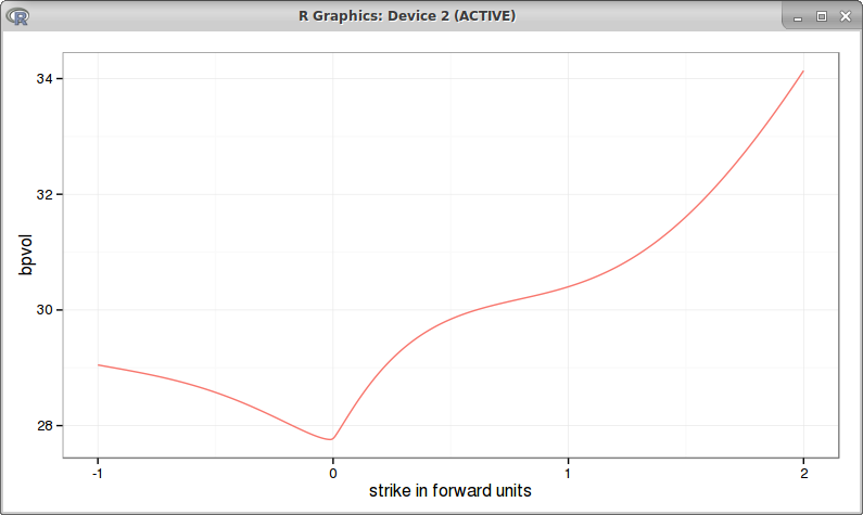
The problem is still there with beta = 0.1:
Overall, the idea of extending SABR to the full real line with the absolute value looks particularly simple, but it's not clear that it makes real financial sense.
There is very little information on variance swaps on a foreign asset. There can be two kinds of contracts:
one that pays the foreign variance in a domestic currency, this is a quanto contract as the exchange rate is implicitly fixed.
one that pays the foreign variance, multiplied by the fx rate at maturity. This is a flexo contract, and is just about buying a variance swap from a foreign bank. The price of such a contract today is very simple, just the standard variance swap price multiplied by the fx rate today (change of measure).
For quanto contracts, it's not so obvious a priori. If we consider a stochastic volatility model for the asset, the replication formula will not be applicable directly as the stochastic volatility will appear in the quanto drift correction. Furthermore, vanilla quanto option prices can not be computed simply as under Black-Scholes, a knowledge of the underlying model is necessary.
Interestingly, under the Schobel-Zhu model, it is simple to fit an analytic formula for the quanto variance swap. The standard variance swap price is:
The quanto variance swap can be priced with the same formula using a slightly different theta:
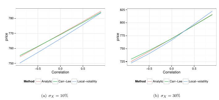
We can use it to assess the accuracy of a naive quanto option replication where we use the ATM quanto forward instead of the forward in the variance swap replication formula.
Interestingly, the quanto forward approximation turns out to be very accurate and the correction is important. The price without correction is the price with zero correlation, and we see it can be +/-5% off in this case.
The local vol price seems a bit off, I am not sure exactly why. It could be due the discretization, the theoretical variance should be divided by (N-1) but here we divide by N where N is the number of observations. That would still lead to a skewed price but better centered around correlation 0.
It's also a bit surprising that local vol is worse than the simpler ATM quanto forward approximation: it seems that it's extracting the wrong information to do a more precise quanto correction, likely related to the shift of stochastic volatility under the domestic measure.
Beside the problem with the discreteness of the replication, variance swaps are sensitive to jumps. This is an often mentioned reason for the collapse of the single name variance swap market in 2008 as jumps are more likely on single name equities.
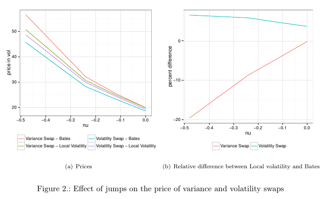
Those graphs are the result of Monte-Carlo simulations with various jump sizes using the Bates model, and using Local Volatility implied from the Bates vanilla prices. The local volatility price will be the same price as per static replication for the variance swap, and we can see it they converge when there is no jump.
The presence of jumps lead to a theoretically higher variance swap price, again, which we miss completely with the static replication. As jumps go higher, the difference is more pronounced.
Volatility swaps are a bit better behaved in this regard. Interestingly, local volatility overestimate the value in this case (which for variance swaps it underestimates the value). I also noticed that the relatively recent formula from Carr-Lee will underestimate jumps even more so than local volatility: it is more precise in the absence of jumps, very close to Heston, but less precise than local volatility when jumps increase in size.
People regularly believe that Variance swaps need to be priced by discrete replication, because the market trades only a discrete set of options.
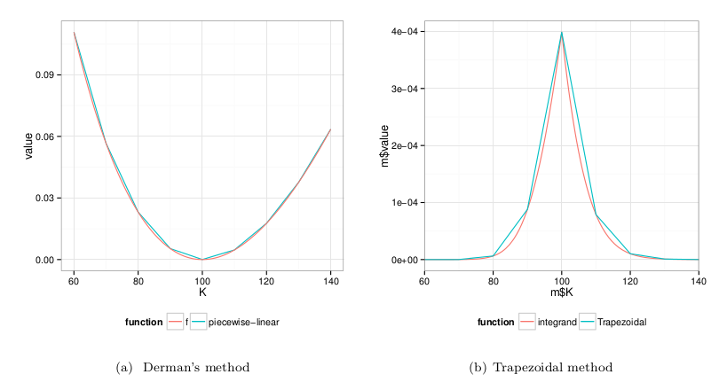
In reality, a discrete replication will misrepresent the tail, and can be quite arbitrary. It looks like the discrete replication as described in Derman Goldman Sachs paper is in everybody's mind, probably because it's easy to grasp. Strangely, it looks like most forget the section "Practical problems with replication" on p27 of his paper, where you can understand that discrete replication is not all that practical.
Reflecting on all of this, I noticed it was possible to create more accurate discrete replications easily, and that those can have vastly different hedging weights. It is a much better idea to just replicate the log payoff continuously with a decent model for interpolation and extrapolation and imply the hedge from the greeks.
It’s quite incredible that Gnome 3.0 was almost an identical mess as KDE 4.0 had been a year or two earlier. Both are much better now, more stable, but both also still have their issues, and don’t feel like a real improvement over Gnome 2.0 or KDE 3.5.
Now the main file manager for Gnome 3.0, Nautilus has buttons with nearly identical icons that mean vastly different things, one is a menu, the other is a list view. Also it does not integrate with other desktops well from a look and feel perpective, here is a screenshot under XFCE (KDE would not look better).The push for window buttons inside the toolbar makes for a funny looking window. In Gnome Shell, it’s not much better, plus there are some windows with a dark theme and some with a standard theme all mixed together.
On the left is Caja: an updated GTK 2.0 version of Nautilus. I find it more functional, I don’t really understand the push to remove most options from the screen in Gnome 3.0. The only positive thing I can see on for the new Nautilus, is the grey color for the left side, which looks more readable and polished.
Interestingly, Nautilus within Ubuntu Unity feels better, it has a real menu and standard looking window. I suppose they customized it quite a bit.
When it comes to HiDPI support, Gnome shell is often touted has having one of the best. Well maybe for laptop screens, but certainly not for larger screens, where it just double everything and everything just looks too big. XFCE is actually decent on HiDPI screens.
In most financial Monte-Carlo simulations, there is the need of generating normally distributed random numbers. One technique is to use the inverse cumulative normal distribution function on uniform random numbers. There are several different popular numerical implementations:
In practice, the most accurate algorithm, AS241, is of comparable speed as the newer but less accurate algorithms of MORO and ACKLAM. Acklam refinement to go to double precision (which AS241 is) kills its performance.
What about the Ziggurat on pseudo rng only? Here are the results with Mersenne-Twister-64, and using the Doornik implementation of the Ziggurat algorithm:
There is a more optimized algorithm, VIZIGNOR, also from Doornik which should be a bit faster. As expected, the accuracy is quite lower than with Sobol, and the Ziggurat looks worse. This is easily visible if one plots the implied volatilities as a function of the spot for AS241 and for ZIGNOR.
AS241 implied volatility on Mersenne-Twister
ZIGNOR implied volatility on Mersenne-Twister
Zignor is much noisier.
Note the slight bump in the scheme EULER-FT-BK that appears because the scheme, that approximates the Broadie-Kaya integrals with a trapeze (as in Andersen QE paper), does not respect martingality that well compared to the standard full truncated Euler scheme EULER-FT, and the slightly improved EULER-FT-MID where the variance integrals are approximated by a trapeze as in Van Haastrecht paper on Schobel-Zhu:
This allows to leak less correlation than the standard full truncated Euler.
In an earlier post, I mentioned the similarities between the Guyon-Labordere particle method and the Vanderstoep-Grzelak-Oosterlee “bin” method to calibrate and price under Local Stochastic volatility. I will be a bit more precise here. The same thing, really
The particle method can be seen as a generalization of the “bin” method. In deed, the bin method consists in doing the particle method using a histogram estimation of the conditional variance. The histogram estimation can be more or less seen as a very basic rectangle kernel with the appropriate bandwidth. The “bin” method is then just the particle method with another kernel (wiki link) (in the particle method, the kernel is a quartic with bandwidth defined by some slightly elaborate formula). A very good paper on this is Silverman Density estimation for statistics and data analysis, referenced by Guyon-Labordere.
In theory, the original particle method has the advantage of using a narrower bandwidth, resulting in a theoretical increase in performance as one does not have to sum over all particles, while providing a more local therefore precise estimate. In practice, the performance advantage is not so clear on my non optimized code. Two-pass There is an additional twist in the particle method: one can compute the expectation and the payoff evaluation in the same Monte-Carlo simulation, or in two sequential Monte-Carlo simulations.
Why would we do two? Mainly because the expectation is computed across all paths, at each time step, while, usually, payoff evaluation requires a full path as it will need to store some state at each observation time for path-dependent payoffs.
We can avoid recomputing the paths by just caching them at each observation time. The problem is that the size of this cache can quickly become extremely large and blow up the memory. For example a 10y daily knock-out will require 10 * 252 * 8 * 2 * MB = 40 GB for 1 million paths.
A side effect of the second simulation is that one can use a Quasi-Random number generator there, while for the first simulation, this is not easy as we compute all paths, dimension by dimension.
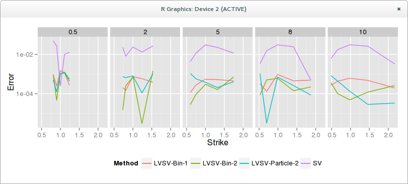
In practice, both methods work well, particle or bins, single-pass or two-pass. Here is a graph of the error in volatility, SV is a not so well calibrated Heston to market data. LVSV are the local stochastic volatility simulations, using as Vanderstoep 100 steps per year and 500K simulations with 30 bins.
The advantages of the particle do not show up in terms of accuracy on this example. I have also noticed that short expiries seem trickier, the error being larger. This might just be due to the time-step size, but interestingly the papers only show graphs of medium (min=6m) to large expiries.