I just stumbled upon this particularly illustrative case where the Crank-Nicolson finite difference scheme behaves badly, and the Rannacher smoothing (2-steps backward Euler) is less than ideal: double one touch and double no touch options.
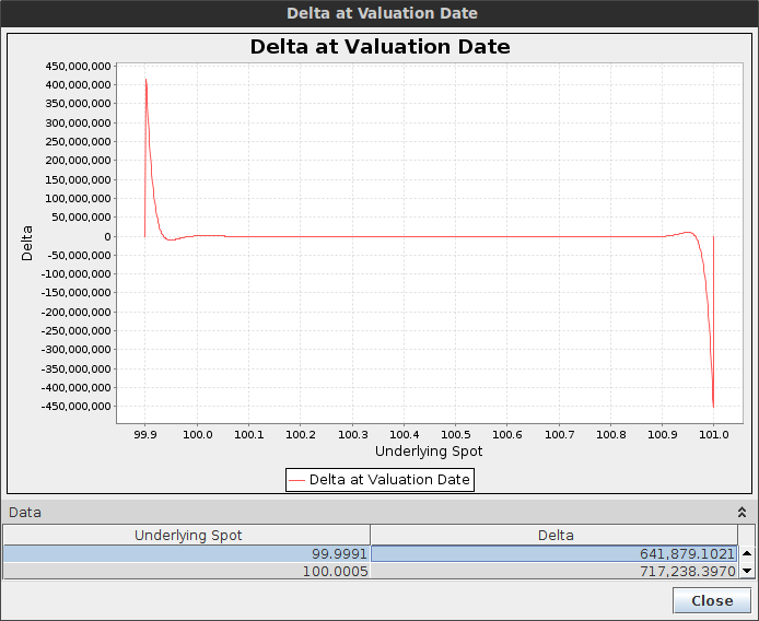
It is particularly evident when the option is sure to be hit, for example when the barriers are narrow, that is our delta should be around zero as well as our gamma. Let's consider a double one touch option with spot=100, upBarrier=101, downBarrier=99.9, vol=20%, T=1 month and a payout of 50K.
Crank-Nicolson shows big spikes in the delta near the boundary
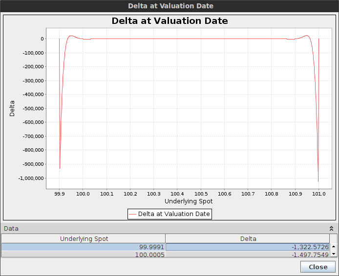
Rannacher shows spikes in the delta as well
Crank-Nicolson spikes are so high that the price is actually a off itself.
The Rannacher smoothing reduces the spikes by 100x but it's still quite high, and would be higher had we placed the spot closer to the boundary. The gamma is worse. Note that we applied the smoothing only at maturity. In reality as the barrier is continuous, the smoothing should really be applied at each step, but then the scheme would be not so different from a simple Backward Euler.
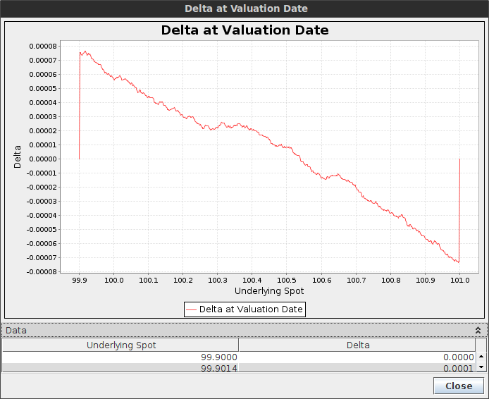
In contrast, with a proper second order finite difference scheme, there is no spike.
Delta with the TR-BDF2 finite difference method - the scale goes from -0.00008 to 0.00008.
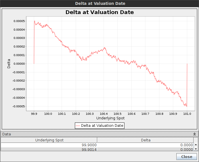
Delta with the Lawson-Morris finite difference scheme - the scale goes from -0.00005 to 0.00005
Both TR-BDF2 and Lawson-Morris (based on a local Richardson extrapolation of backward Euler) have a very low delta error, similarly, their gamma is very clean. This is reminiscent of the behavior on American options, but the effect is magnified here.
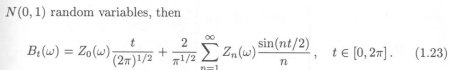
I was wondering how to generate some nice cloudy like texture with a simple program. I first thought about using the Brownian motion, but of course if one uses it raw, with one pixel representing one movement in time, it's just going to look like a very noisy and grainy picture like this:
Normal noise
There is however a nice continuous representation of the Brownian motion : the Paley-Wiener representation
This can produce an interesting smooth pattern, but it is just 1D. In the following picture, I apply it to each row (the column index being time), and then for each column (the row index being time). Of course this produces a symmetric picture, especially as I reused the same random numbers
If I use new random numbers for the columns, it is still symmetric, but destructive rather than constructive.
It turns out that spatial processes are something more complex than I first imagined. It is not a simple as using a N-dimensional Brownian motion, as it would produce a very similar picture as the 1-dimensional one. But this paper has a nice overview of spatial processes. Interestingly they even suggest to generate a Gaussian process using a Precision matrix (inverse of covariance matrix). I never thought about doing such a thing and I am not sure what is the advantage of such a scheme.
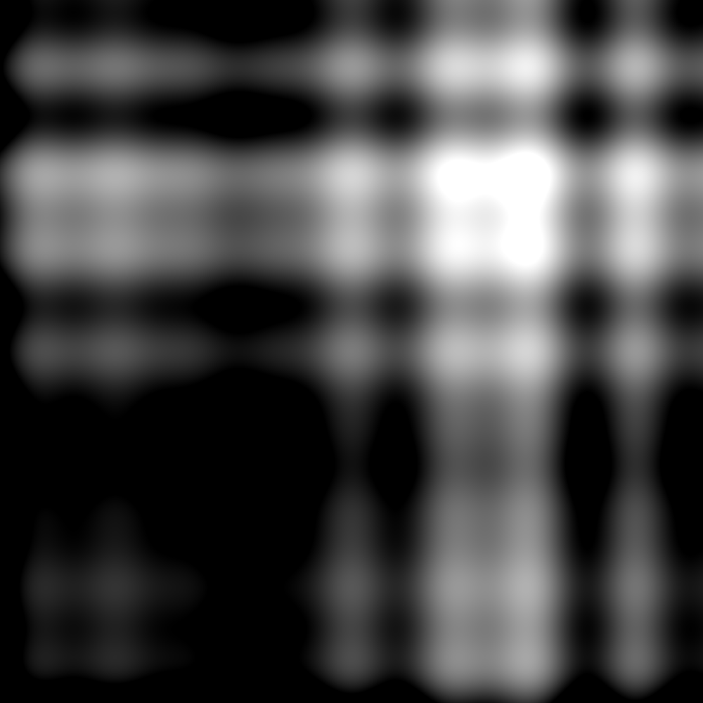
There is a standard graphic technique to generate nice textures, originating from Ken Perlin for Disney, it is called simply Perlin Noise. It turns out that several web pages in the top Google results confuse simple Perlin noise with fractal sum of noise that Ken Perlin also helped popularize (see his slides: standard Perlin noise, fractal noise). Those pages also believe that the later is simpler/faster. But there are two issues with fractal sum of noise: the first one is that it relies on an existing noise function - you need to first build one (it can be done with a random number generator and an interpolator), and the second one is that it ends up being more complex to program and likely to evaluate as well, see for example the code needed here. The fractal sum of noise is really a complementary technique.
The insight of Perlin noise is to not generate random color values that would be assigned to shades of grey as in my examples, but to generate random gradients, and interpolate on those gradient in a smooth manner. In computer graphics they like the cosine function to give a little bit of non-linearity in the colors. A good approximation, usually used as a replacement in this context is 3x^2 - 2x^3. It's not much more complicated than that, this web page explains it in great details. It can be programmed in a few lines of code.
very procedural and non-optimized Go code for Perlin noise
I have looked a few months ago already at Julia, Dart, Rust and Scala programming languages to see how practical they could be for a simple Monte-Carlo option pricing.
I forgot the Go language. I had tried it 1 or 2 years ago, and at that time, did not enjoy it too much. Looking at Go 1.5 benchmarks on the computer language shootout, I was surprised that it seemed so close to Java performance now, while having a GC that guarantees pauses of less 10ms and consuming much less memory.
I am in general a bit skeptical about those benchmarks, some can be rigged. A few years ago, I tried my hand at the thread ring test, and found that it actually performed fastest on a single thread while it is supposed to measure the language threading performance. I looked yesterday at one Go source code (I think it was for pidigits) and saw that it just called a C library (gmp) to compute with big integers. It’s no surprise then that Go would be faster than Java on this test.
So what about my small Monte-Carlo test?
Well it turns out that Go is quite fast on it:
Multipl.
Rust
Go
1
0.005
0.007
10
0.03
0.03
100
0.21
0.29
1000
2.01
2.88
It is faster than Java/Scala and not too far off Rust, except if one uses FastMath in Scala, then the longest test is slighly faster with Java (not the other ones).
There are some issues with the Go language: there is no operator overloading, which can make matrix/vector algebra more tedious and there is no generic/template. The later is somewhat mitigated by the automatic interface implementation. And fortunately for the former, complex numbers are a standard type. Still, automatic differentiation would be painful.
Still it was extremely quick to grasp and write code, because it’s so simple, especially when compared to Rust. But then, contrary to Rust, there is not as much safety provided by the language. Rust is quite impressive on this side (but unfortunately that implies less readable code). I’d say that Go could become a serious alternative to Java.
I also found an interesting minor performance issue with the default Go Rand.Float64, the library convert an Int63 to a double precision number this way:
The reasoning behind this later code is that the mantissa is 52 bits, and this is the most accuracy we can have between 0 and 1. There is no need to go further, this also avoids the issue around 1. It’s also straightforward that is will preserve the uniform property, while it’s not so clear to me that r.Int63()/2^63 is going to preserve uniformity as double accuracy is higher around 0 (as the exponent part can be used there) and lesser around 1: there is going to be much more multiple identical results near 1 than near 0.
It turns out that the if check adds 5% performance penalty on this test, likely because of processor caching issues. I was surprised by that since there are many other ifs afterwards in the code, for the inverse cumulative function, and for the payoff.
In his book "Monte Carlo Methods in Finance", P. Jäckel explains a simple way to clean up a correlation matrix. When a given correlation matrix is not positive semi-definite, the idea is to do a singular value decomposition (SVD), replace the negative eigenvalues by 0, and renormalize the corresponding eigenvector accordingly.
One of the cited applications is "stress testing and scenario analysis for market risk" or "comparative pricing in order to ascertain the extent of correlation exposure for multi-asset derivatives", saying that "In many of these cases we end up with a matrix that is no longer positive semi-definite".
It turns out that if one bumps an invalid correlation matrix (the input), that is then cleaned up automatically, the effect can be a very different bump. Depending on how familiar you are with SVD, this could be more or less obvious from the procedure,
As a simple illustration I take the matrix representing 3 assets A, B, C with rho_ab = -0.6, rho_ac = rho_bc = -0.5.
For those rho_ac and rho_bc, the correlation matrix is not positive definite unless rho_ab in in the range (-0.5, 1). One way to verify this is to use the fact that positive definiteness is equivalent to a positive determinant. The determinant will be 1 - 2*0.25 - rho_ab^2 + 2*0.25*rho_ab.
It turns out that rho_bc has changed by only 0.66% and rho_ac by -0.30%, rho_ab by -0.34%. So our initial bump (0,0,1) has been translated to a bump (-0.34, -0.30, 0.66). In other words, it does not work to compute sensitivities.
One can optimize to obtain the nearest correlation matrix in some norm. Jaeckel proposes a hypersphere decomposition based optimization, using as initial guess the SVD solution. Higham proposed a specific algorithm just for that purpose. It turns out that on this example, they will converge to the same solution (if we use the same norm). I tried out of curiosity to see if that would lead to some improvement. The first matrix becomes
We find back the same issue, rho_bc has changed by only 0.67%, rho_ac by -0.31% and rho_ab by -0.33%. We also see that the SVD correlation or the real near correlation matrix are quite close, as noticed by P. Jaeckel.
Of course, one should apply the bump directly to the cleaned up matrix, in which case it will actually work as expected, unless our bump produces another non positive definite matrix, and then we would have correlation leaking a bit everywhere. It's not entirely clear what kind of meaning the risk figures would have then.
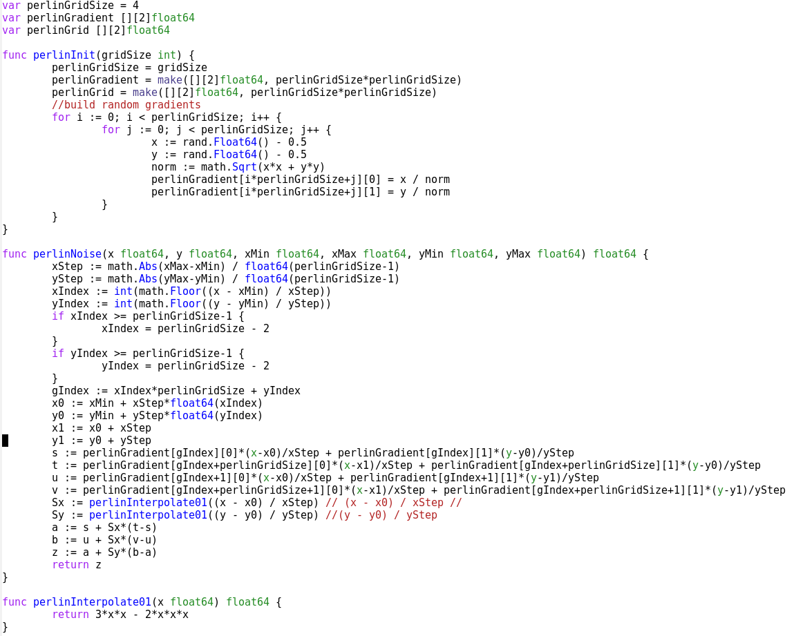
There are not many arbitrage free extrapolation schemes. Benaim et al. extrapolation is one of the few that claims it. However, despite the paper’s title, it is not truely arbitrage free. The density might be positive, but the forward is not preserved by the implied density. It can also lead to wings that don’t obey Lee’s moments condition.
On a Wilmott forum, P. Caspers proposed the following counter-example based on extrapolating SABR: \( \alpha=15%, \beta=80%, \nu=50%, \rho=-48%, f=3%, T=20.0 \). He cut this smile at 2.5% and 6% and used the BDK extrapolation scheme with mu=nu=1.
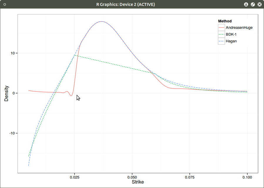
A truly arbitrage free extrapolation can be obtained through Andreasen Huge volatility interpolation, making sure the grid is wide enough to allow extrapolation. Their method is basically a one step finite difference implicit Euler scheme applied to a local volatility parameterization that has as many parameters than prices. The method is presented with piecewise constant local volatility, but actually used with piecewise linear local volatility in their example.
Smile.
Density with piecewise linear local volatility.
There is still a tiny oscillation that makes the density negative, but one understands why typical extrapolations fail on the example: the change in density must be very steep.
Note that moving the left extrapolation point even closer to the forward might fix BDK negative density, but we are already very close, and we can really wonder if going closer is really a good idea since we would effectively use a somewhat arbitrary extrapolation in most of the interpolation zone.
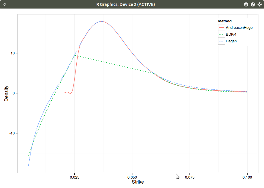
It turns out that we can also use a cubic spline local volatility with linear extrapolation, and the density would look then:
Density with cubic spline local volatility.
Interestingly, the right side of the density is much better captured.
The wiggle persists, although it is smaller. This is likely due to the fact that I am using a cubic spline on top of the finite difference prices (in order to have a C2 density). Using a better C2 convexity preserving interpolation would likely remove this artefact.
Those figures also show why relying just on extrapolation to fix SABR is not necessarily a good idea: even a real arbitrage free extrapolation will make a not so meaningful density. The proper solution is to really use Hagan’s arbitrage free SABR PDE, which would be as nearly fast in this case.
I am looking at various extrapolation schemes of the implied volatilities. An interesting one I stumbled upon is due to Kahale. Even if his paper is on interpolation, there is actually a small paragraph on using the same kind of function for extrapolation. His idea is to simply lookup the standard deviation \( \Sigma \) and the forward \(f\) corresponding to a given market volatility and slope:
$$ c_{f,\Sigma} = f N(d_1) - k N(d_2)$$
with
$$ d_1 = \frac{\log(f/k)+\Sigma^2 /2}{\Sigma} $$
We have simply:
$$ c’(k) = - N(d_2)$$
He also proves that we can always find those two parameters for any \( k_0 > c_0 > 0, -1 < c_0’ < 0 \)
Then I had the silly idea of trying to match with a put instead of a call for the left wing (as those are out-of-the-money, and therefore easier to invert numerically). It turns out that it works in most cases in practice and produces relatively nice looking extrapolations, but it does not always work. This is because contrary to the call, the put value is bounded with \(f\).
$$ p_{f,\Sigma} = k N(-d_2) - f N(-d_1)$$
Inverting \( p_0’ \) is going to lead to a specific \( d_2 \), and you are not guaranteed that you can push \( f \) high and have \( p_{f, \Sigma} \) large enough to match \( p_0 \). As example we can just take \(p_0 \geq k N(-d_2)\) which will only be matched if \( f \leq 0 \).
This is slightly unintuitive as put-call parity would suggest some kind of equivalence. The problem here is that we would need to consider the function of \(k\) instead of \(f\) for it to work, so we can’t really work with a put directly.
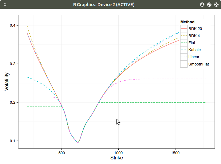
Here are the two different extrapolations on Kahale own example:
Window Extrapolation of the left wing with calls (blue doted line)
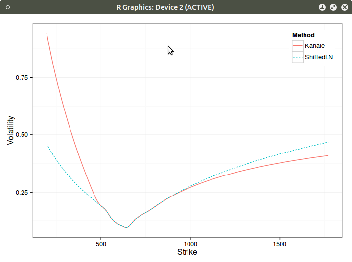
Extrapolation of the left wing with puts (blue doted line)
Displaced diffusion extrapolation is sometimes advocated. It is not the same as Kahale extrapolation: In Kahale, only the forward variable is varying in the Black-Scholes formula, and there is no real underlying stochastic process. In a displaced diffusion setting, we would adjust both strike and forward, keeping put-call parity at the formula level. But unfortunately, it suffers from the same kind of problem: it can not always be solved for slope and price. When it can however, it will give a more consistent extrapolation.
I find it interesting that some smiles can not be extrapolated by displaced diffusion in a C1 manner except if one allows negative volatilities in the formula (in which case we are not anymore in a pure displaced diffusion setting).
Extrapolation of the left wing using negative displaced diffusion volatilities (blue dotted line)
sometimes (rarely) my laptop would not wake up from sleep.
notifications sometimes keep popping up too much.
on my desktop, experienced strong tearing issues with the Radeon graphic card, except with some very specific combination of video player settings and desktop settings (and then I had annoying redraw issue when pushing volume up/down in movies).
I am satisfied with two different approaches since:
OpenSuse 13.2 with KDE 4. I use that on my desktop, all issues are gone, and the integration of KDE in OpenSuse is clearly the best I have experienced. In contrast, KDE 5 on Ubuntu was a disaster for me. I also managed to fuck up the apt dependencies so much that I thought it would be simpler to reinstall a new distribution.
Mate on Ubuntu 15.04. Very impressed so far. It’s probably what Gnome should have been instead of going to 3.0. Even if there are nice aspects of the Gnome shell, Mate is fast, pretty, user friendly, much better than Cinnamon. There are even a few layouts to choose (most of them are good), here is “Eleven with Mate menu” (it installed and setup the Plank dock automatically for that layout, more traditional layouts without dock are available):
C. Reisinger kindly pointed out to me this paper around square root Crank-Nicolson. The idea is to apply a square root of time transformation to the PDE, and discretize the resulting PDE with Crank-Nicolson. Two reasons come to mind to try this:
the square root transform will result in small steps initially, where the solution is potentially not so smooth, making Crank-Nicolson behave better.
it is the natural time of the Brownian motion.
Interestingly, it has nicer properties than what those reasons may suggest. On the Fokker-Planck density PDE, it does not oscillate under some very mild conditions and preserves density positivity at the peak.
Out of curiosity I tried it to price a one touch barrier option. Of course there is an analytical solution in my test case (Black-Scholes assumptions), but as soon as rates are assumed not constant or local volatility is used, there is no other solution than a numerical method. In the later case, finite difference methods are quite good in terms of performance vs accuracy.
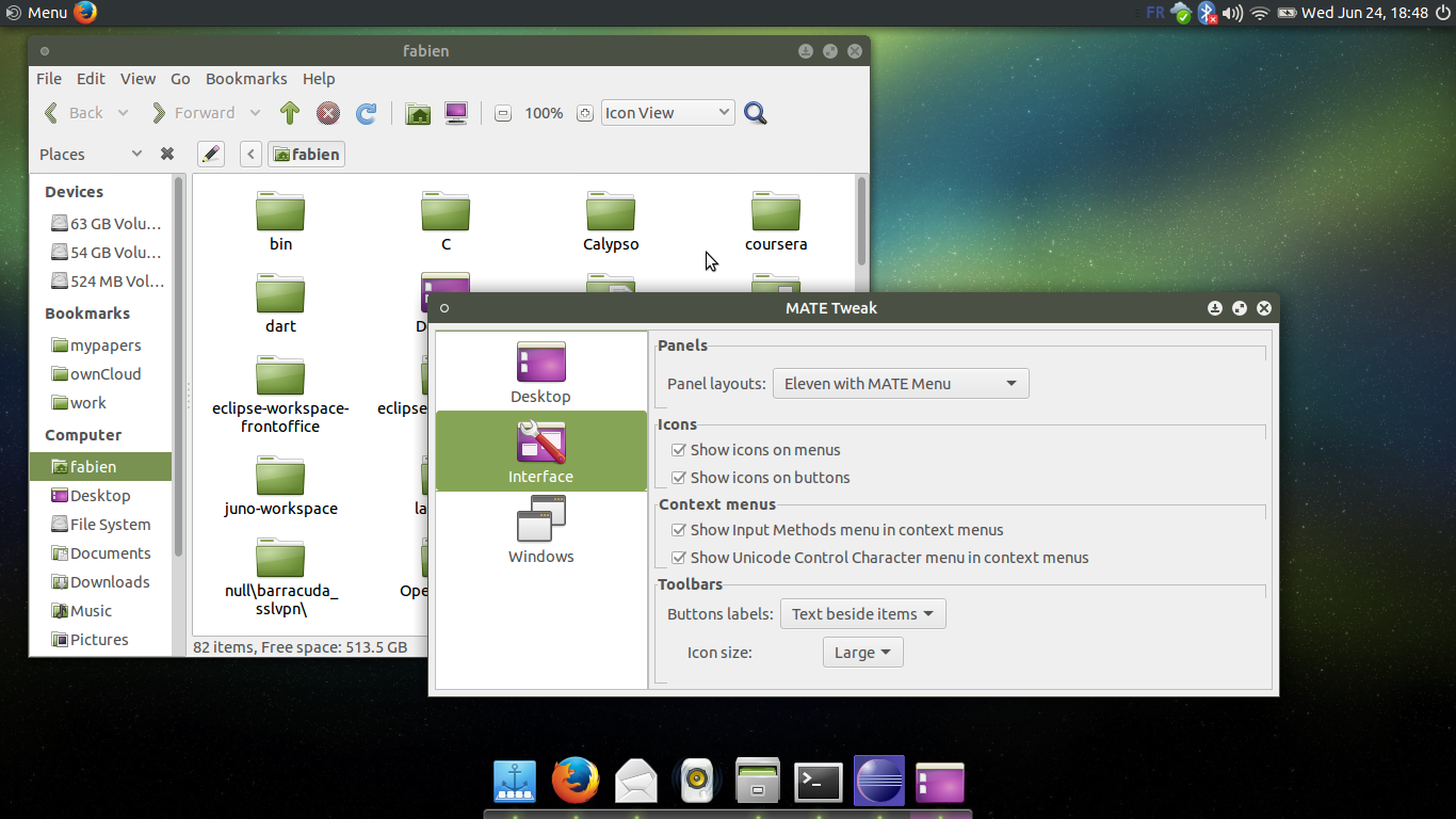
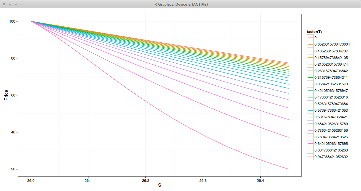
The classic Crank-Nicolson gives a reasonable price, but the strong oscillations near the barrier, at every time step are not very comforting.
Crank-Nicolson Prices near the Barrier. Each line is a different time.
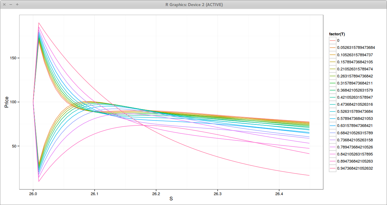
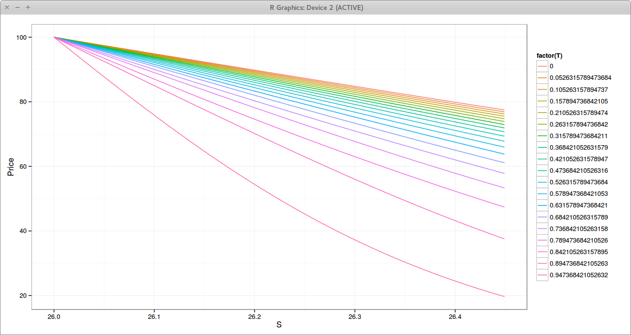
Moving to square root of time removes nearly all oscillations on this problem, even with a relatively low number of time steps compared to the number of space steps.
Square Root Crank-Nicolson Prices near the Barrier. Each line is a different time.
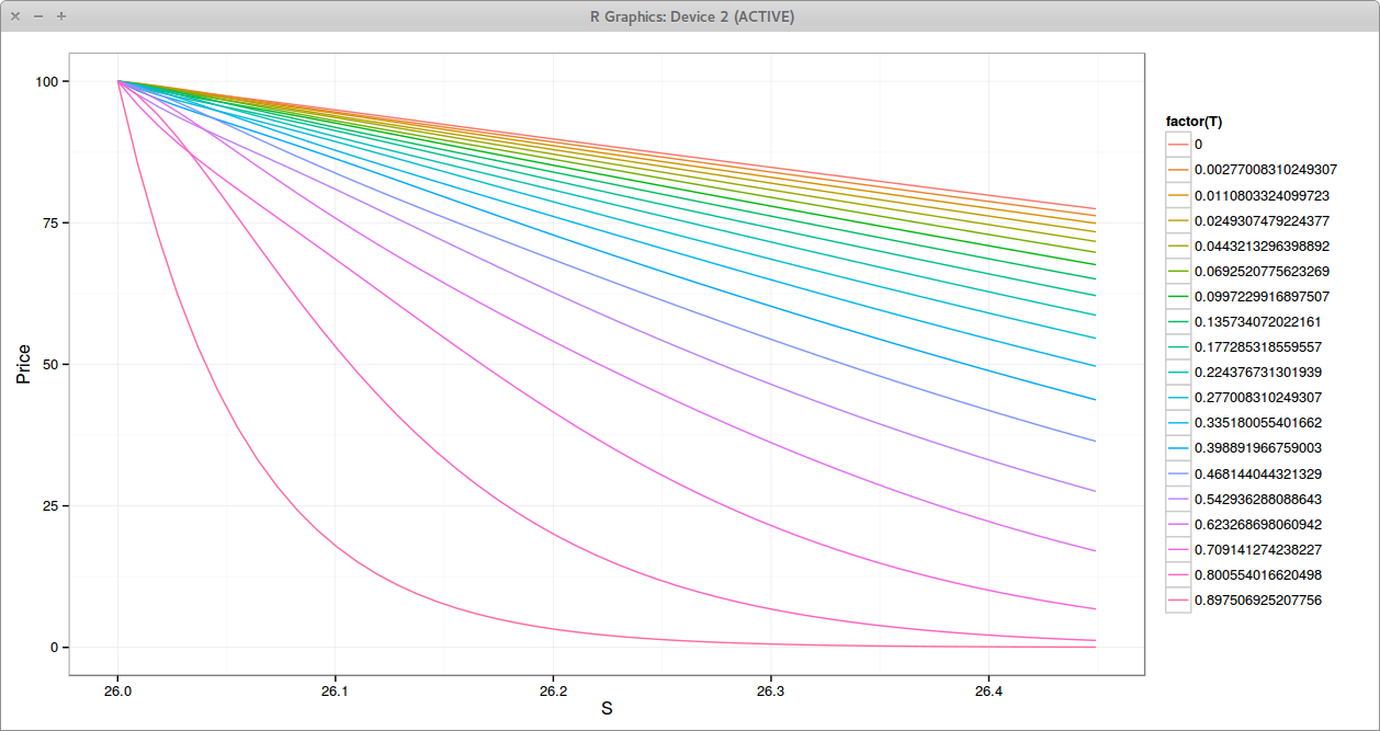
We can see that the second step prices are a bit higher than the third step (the lines cross), which looks like a small numerical oscillation in time, even if there is no oscillation is space.
TR-BDF2 Prices near the Barrier. Each line is a different time.
As a comparison, the TR-BDF2 scheme does relatively well: oscillations are removed after the second step, even with the extreme ratio of time steps vs space steps used on this example so that illustrations are clearer - Crank-Nicolson would still oscillate a lot with 10 times less space steps but we would not see oscillation on the square root Crank-Nicolson and a very mild one on TR-BDF2.
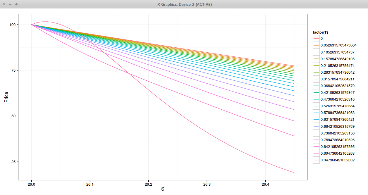
The LMG2 scheme (a local richardson extrapolation) does not oscillate at all on this problem but is the slowest:
LMG2 Prices near the Barrier. Each line is a different time.
The square root Crank-Nicolson is quite elegant. It can however not be applied to that many problems in practice, as often some grid times are imposed by the payoff to evaluate, for example in a case of a discrete weekly barrier. But for continuous time problems (density PDE, Vanilla, American, continuous barriers) it's quite good.
In reality, with a continuous barrier, the payoff is not discontinuous at every step, but it is only discontinuous at the first step. So Rannacher smoothing would work very well on that problem:
Rannacher Prices near the Barrier. Each line is a different time.
The somewhat interesting payoff left for the square root Crank-Nicolson is the American.
Here are the main steps of Hagan derivation. Let's recall his notation for the SABR model where typically, \\(C(F) = F^\beta\\)
First, he defines the moments of stochastic volatility:
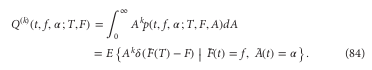
Then he integrates the Fokker-Planck equation over all A, to obtain
On the backward Komolgorov equation, he applies a Lamperti transform like change of variable:
And then makes another change of variable so that the PDE has the same initial conditions for all moments:
This leads to
It turns out that there is a magical symmetry for k=0 and k=2.
Note that in the second equation, the second derivative applies to the whole.
Because of this, he can express \\(Q^{(2)}\\) in terms of \\(Q^{(0)}\\):
And he plugs that back to the integrated Fokker-Planck equation to obtain the arbitrage free SABR PDE:
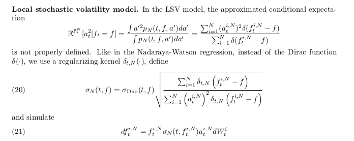
There is a simple more common explanation in the world of local stochastic volatility for what's going on. For example, in the particle method paper from Guyon-Labordère, we have the following expression for the true local volatility.
In the first equation, the numerator is simply \(Q^{(2)}\) and the denominator \(Q^{(0)}\). Of course, the integrated Fokker-Planck equation can be rewritten as:
Karlsmark uses that approach directly in his thesis, using the expansions of Doust for \(Q^{(k)}\). Looking a Doust expansions, the fraction reduces straightforwardly to the same expression as Hagan, and the symmetry in the equations appears a bit less coincidental.
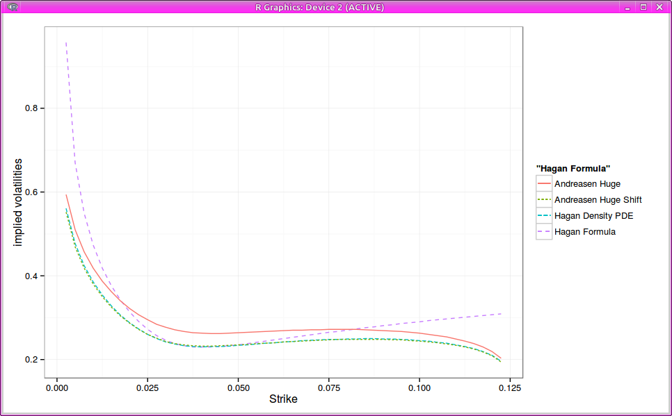
I looked nearly two years ago already at the arbitrage free SABR of Andreasen-Huge in comparison to the arbitrage free PDE of Hagan and showed how close the ideas were: Andreasen-Huge relies on the normal Dupire forward PDE using a slightly simpler local vol (no time dependent exponential term) while Hagan works directly on the Fokker-Planck PDE (you can think of it as the Dupire Forward PDE for the density) and uses an expansion of same order as the original SABR formula (which leads to an additional exponential term in the local volatility).
One clever idea from Andreasen-Huge is the use of a single step. It turns out that their idea is not completely new. Daniel Duffy sent me some old papers from Shishkin around fitted schemes (here is one). This is very much the same thing, except Shishkin concern is about a good handling of discontinuity in the initial condition, and therefore makes the association step function => cumulative density to fit the diffusion parameter. Andreasen-Huge work directly with the call prices as this is what they solve.
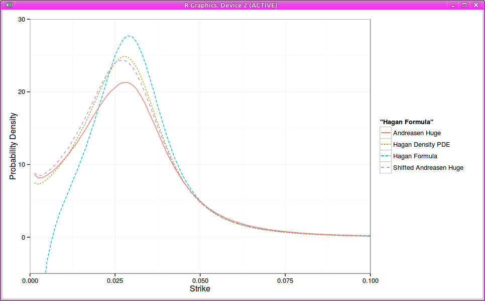
One drawback of Andreasen-Huge one step method is the inability to match the standard SABR smile: the parameters don’t have exactly the same meaning. It turns out that by just shifting proportionally the local volatility by a constant factor, Andreasen Huge matches Hagan PDE vols quite closely.
Implied Black volatilities
Probability density
While this is interesting in itself, it’s still not so simple to backup this factor without solving for it (and then the method looses appeal).