In my paper “Fast and Accurate Analytic Basis Point Volatility”,
I use a table of Chebyshev polynomials to provide an accurate representation of some function. This is
an idea I first saw in the Faddeeva package to
represent the cumulative normal distribution with high accuracy, and high performance. It is also
simple to find out the Chebyshev polynomials, and which intervals are the most appropriate for those, which
makes this technique quite appealing.
Still, it would have been nice to have also a more visually appealing rational function representation, as W. Shaw
did for the cumulative normal distribution (again). Popular algorithms to find the best rational function representation
seem to be minimax or Remez. But I could not find an open-source library where those were implemented. There is an
interesting implementation in chebfun but this depends on Matlab.
The Numerical recipe book provides a simple algorithm in chapter 5.13, not looking for the best possible rational function, but just for one
that would be “good enough”. Interestingly, the first part of the algorithm merely computes a least squares solution
on some chebyshev like nodes. I however quickly noticed funny behaviors with the code: it could produce a worse fit
for a higher order numerator or denominator. Then I tried some least squares python code which ended up being just buggy:
I am not sure what the code actually does with all the numpy and scipy magic, it gives solutions with poles in the data, and clearly not the least squares solution. I can’t fully understand why one would propose such a code.
It turns out that I had an alternative very basic least squares polynomial fit implementation, which is based on this matrix representation.
I wondered if it would be as prone to errors as Numerical recipe code (where they use SVD internally to solve).
The answer is: it depends. It depends on the solver used. If I use a QR solver, then the implementation looks robust on my test data,
much more than Numerical recipe code. If I use LU, it just fails in some cases. If I use SVD, it is sometimes better sometimes worse than Numerical recipe.
Interestingly, I thought, that, maybe, a gradient descent could allow to regain the lost accuracy with SVD, using
as starting point, the SVD guess. However, it does not work, it just converges more or less to the same (bad) solution.
Another interesting point, is that the using QR decomposition (instead of SVD)
in the Numerical recipe implementation resulted in a much better solution, better even than my basic least squares fit,
which looked robust, but was actually not so much.
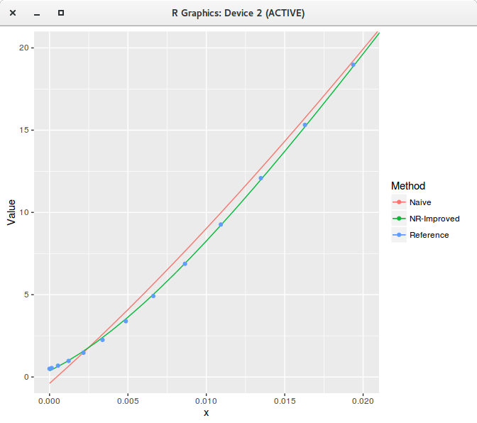
Armed with this improved Numerical recipe code (labeled NRI), here is a comparison of fit of my naive code (with QR) against the improved numerical recipe
(NRI) for a polynomial of degree 20. We can visually see the difference (when we zoom)!
Least squares polynomial fit of degree 20 zoomed.
The RMSE difference on the full interval [0,1] on 1000 equidistant points is huge:
Method
RMSE
Polynomial Naive
0.234
Polynomial NRI
0.039
Rational NRI
0.001
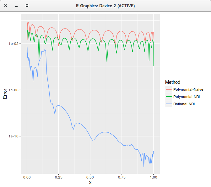
A 10/10 rational function (numerator of degree 10, denominator of degree 10) gives a much better fit than a polynomial of degree 20. It is interesting to look at the error
visually to understand how large is the difference:
Least squares polynomial fit error of degree 20.
I still can draw a conclusion to my quest for a rational function approximation: I won’t find a good one with the
change of variables I am using in my paper, as I would imagine the least squares solution to be at worst around one order of magnitudes
away from the minimax. The errors I got suggest I would need a few rational functions, maybe 3 or more, and then it does not look
all that appealing compared to the table of Chebyshev polynomials.
I thought this was a good example of how relatively simple numerical tasks can be challenging in practice.
Update - The paper now contains a solution for the normal volatility inversion problem with only 3 rational functions.
I am experimenting a bit with least squares splines. Existing algorithms (for example from the NSWC Fortran library) usually work
with B-splines, a relatively simple explanation of how it works is given in this paper (I think this is how De Boor coded it in the NSWC library).
Interestingly there is an equivalent formulation in terms of standard cubic splines, although it seems that the
pseudo code on that paper has errors.
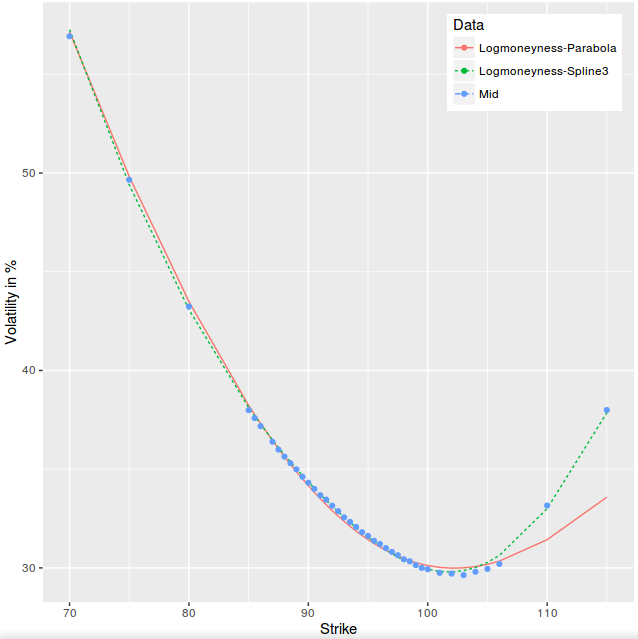
Least squares splines give a very good fit for option implied volatilities with only a few parameters.
In theory, the number of parameters is N+2 where N is the number of interpolation points.
I tried on some of my AAPL 1 month option chain, with only 3 points (so 2 splines or 5 free parameters).
least squares spline on 1m AAPL options.
It would be interesting to add the natural constraints so that it can be linearly extrapolated. Maybe for next time.
I recently had some fun trying to work directly with the option chain from the Nasdaq website.
The data there is quite noisy, but a simple parabola can still give an amazing fit. I will consider the options of maturity two years as illustration.
I also relied on a simple implied volatility algorithm that can be summarized in the following steps:
Compute a rough guess for the forward price by using interest, borrow curves and by extrapolating the dividends.
Imply the forward from the European Put-Call parity relationship on the mid prices of the two strikes closes to the rough forward guess. A simple linear interpolation between the two strikes can be used to compute the forward.
Compute the Black implied volatilities as if the option were European using P. Jaeckel algorithm.
Calibrate the proportional dividend amount or the growth rate by minimizing, for example with a Levenberg-Marquardt minimizer, the difference between model and mid-option prices corresponding to the three strikes closest to the forward. The parameters in this case are effectively the dividend amount and the volatilities for Put and Call options (the same volatility is used for both options). The initial guess stems directly from the two previous steps. American option prices are computed by the finite difference method.
Solve numerically the volatilities one by one with the TOMS748 algorithm so that the model prices match the market mid out-of-the-money option prices.
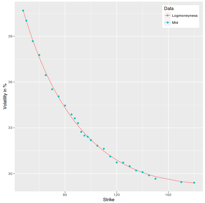
Then I just fit a least squares parabola in variance on log-moneyness, using options trading volumes as weights and obtain the following figure:
least squares parabola on 2y AAPL options.
Isn’t the fit just amazing?
Even if I found it surprising, it’s probably not so surprising. The curve has to be smooth, somewhat monotone, and will be therefore like a parabola near the money. While there is no guarantee it will fit that well far away, it’s actually a matter of scale. Short maturities will lead to not so great fit in the wings, while long maturities will correspond to a narrower range of scaled strikes and match better a parabola.
The option chain on Yahoo finance shows an implied volatility number for each call or put option in the last column.
I was wondering a bit how they computed that number. I did not exactly find out their methodology, especially since we don’t even know the daycount convention used, but
I did find that it was likely just garbage.
A red-herring is for example the large discrepancy between put vols and call vols. For example strike 670, call vol=50%, put vol=32%.
This suggests that the two are completely decoupled, and they use some wrong forward (spot price?) to obtain those numbers. If I compute
the implied volatilities using put-call parity close to the money to find out the implied forward price, I end up with ask vols of 37% and 34% or call and put mid vols of 33%.
By considering the put-call parity, I assume European option prices, which is not correct in this case. It turns out however, that with the low interest rates we live in, there is nearly zero additional value due to the American early exercise.
I am not sure what use people can have of Yahoo implied volatilities.
Tufte proposes interesting guidelines to present data, or even to design written semi-scientific papers or books. Some advices
are particularly relevant like the careful use of colors (don’t use all the colors of the rainbow just because you can), and
in general don’t add lines in a graph or designs that are not directly relevant to the message that needs to be conveyed. There is also a parallel
with Feynman message against (Nasa) Powerpoint presentations. But other inspirations, are somewhat doubtful.
He seems to have a fetish for old texts. They might be considered pretty, or interesting in some ways, but
I don’t find them particularly easy to read. They look more like esoteric books rather than practical books. If you want to write
the new Bible for your new cult, it’s probably great, not so sure it’s so great for a more simple subject.
Also somewhat surprisingly, his own website is not very well designed, it looks like a maze and very end of 90s.
I experimented a bit with the Tufte latex template. It produced that document for example. But someone rightfully pointed out to me
that the reference style was not really elegant, that it did not look like your typical nice science paper references. Furthermore,
using superscript so much could be annoying for someone used to read math and consider superscript numbers as math symbols.
In general, there seems to be a conflict between the use of Latex and many Tufte guidelines:
Latex does not encourage you to lay out one by one each piece,
something the good old desktop publishing software allow you to do quite well.
I was also wondering a bit on what design to use for a book. And I realised that the best layout to consider is simply the layout
of a book I enjoyed to read. For example, I like the recent SIAM book design, I find that it gives enough space to read the text
and the maths without having the impression of deciphering some codex, and without headache. It turns out there is even a latex template available.
When the dividend curve is built from discrete cash dividends, the dividend yield is discontinuous at the dividend time as the asset price jumps from the dividend amount.
This can be particularly problematic for numerical schemes like finite difference methods. In deed, a finite difference grid
will make use of the forward yield (eventually adjusted to the discretisation scheme), which explodes then.
Typically, if one is not careful about this, then increasing the number of time steps does not increase accuracy anymore, as
the spike just becomes bigger on a smaller time interval. A simple work-around is to limit the resolution to one day.
This means that intraday, we interpolate the dividend yield.
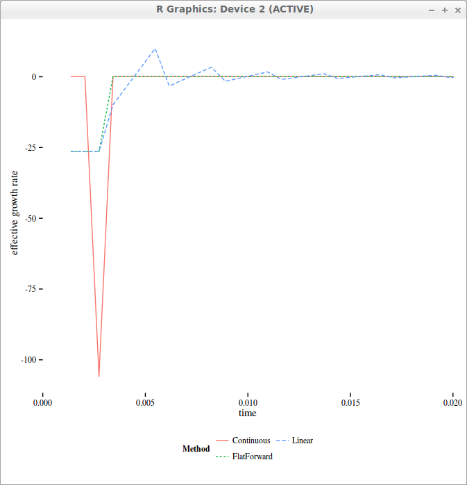
If we simply interpolate the yields linearly intraday, then the yield becomes continuous again, and numerical schemes will work much better.
But if we take a look at the actual curve of “forward” yields, it becomes sawtooth shaped!
effective forward drift used in the finite difference grid with 4 time-steps per day
On the above figure, we can see the Dirac like forward yield if we work with the direct formulas, while interpolating intraday allows to smooth out the initial Dirac overall the interval corresponding to 1-day.
In reality, one should use flat forward interpolation instead, where the forward yield is maintained constant during the day. The forward rate is defined as
where the continuously compounded rate \(r\) is defined so that \(Z(0,t)= e^{-r(t)t}\).
In the case of the Black-Scholes drift, the drift rate is defined so that the forward price (not to confuse with the forward rate) \(F(0,t)= e^{-q(t)t}\).
The flat forward interpolation is equivalent to a linear interpolation on the logarithm of discount factors.
In ACT/365, let \(t_0=\max\left(0,\frac{365}{\left\lceil 365 t \right\rceil-1}\right), t_1 = \frac{365}{\left\lceil 365 t \right\rceil}\), the interpolated yield is:
I moved my blog from blogger to Hugo. Blogger really did not evolve since Google take-over in 2003. Wordpress is today much nicer and prettier. It’s clear that Google did not invest at all, possibly because blogs are passé. Compared to mid 2000, there are very few blogs today. Even programming blogs are scarce. It could be interesting to quantify this. My theory is that it is the direct consequence of the popularity of social networks, and especially facebook (possibly also stackoverflow for programmers): people don’t have time anymore to write as their extra-time is used on social networks. Similarly I noticed that almost nobody comments anymore to the point that even Disqus is very rarely used, and again I attribute that to the popularity of sites like reddit. This is why I did not bother with a comment section on my blog, just email me or tweet about it instead.
I was always attracted by the static web sites concept, because there is actually very little things that ought to be truely dynamic from a individual point of view. Dynamic hosting also tends to be problematic in the long-run, for example I never found the time to upgrade my chord search engine to the newer Google appengine and now it’s just off. I used to freeze my personal website (created with a dynamic templating tool Velocity, django, etc.) with a python script. So a static blog was the next logical step, and these days, it’s quite popular. Static blogs put the author fully in control of the content and its presentation. Jekyll started the trend along with github allowing good old personal websites. It offers a modern looking blog, with very little configuration steps. I tried Hugo instead because it’s written in the Go language. It’s much faster, but I don’t really care about that for something of the size of my blog. I was curious however how good was the Go language on real world projects, and I knew I could always customize it if I ever needed to. Interestingly, I did stumble on a few panics (core dump equivalent where the program just crashes, in this case the hugo local server), something that does not happen with Java based tools or even with Ruby or Python based tools. Even though I like the Go language more and more (I am doing some pet project with it - I believe in the focus on fast compilation and simple language), I found this a bit alarming. This is clearly a result of the errors versus exceptions choice, as it’s up to the programmer to handle the errors properly and not panic unnecessarily (I even wonder if it makes any sense to panic for a server).
Anyway I think it looks better now, maybe a bit too minimalist. I’ll add details when I have more time.
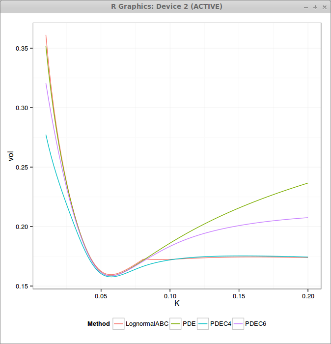
On the Wilmott forum, Pat Hagan has recently suggested to cap the equivalent local volatility in order to control the wings and better match CMS prices. It also helps making the SABR approximation better behaved as the expansion is only valid when
While it is straightforward to include in the PDE, it is more difficult to derive a good approximation. The zero-th order behaves as expected, but the first order formula has a unnatural kink, likely because of the non differentiability due to the min function.
The following graphs presents the non capped PDE, the capped PDE with M=4*nu (PDEC4) and M=6*nu (PDEC6) as well as the approximation (Andersen Ratcliffe / Gatheral first order) where I have only taken care of the right wing. The SABR parameters are alpha = 0.0630, beta = 0.7, rho = -0.363, nu = 0.421, T = 10, f = 0.0439.
We can see that the higher the cap is, the closer we are to the standard SABR PDE, and the lower the cap is, the flatter are the wings.
The approximation matches well ATM (it is then equivalent to standard SABR PDE) but then has a discontinuous derivative for the K that reaches the threshold M. Far away, it matches very well again.
There is something funny going on with upcoming generic top level domains (gTLDs), they seem to be looked up in a strange manner (at least on latest Linux). For example:
ping chrome
or
ping nexus
returns 127.0.53.53.
While existing official gTLDs don't (ping dental returns "unknown host" as expected). I first thought it was a network misconfiguration, but as I am not the only one to notice this, it's likely a genuine internet issue.
I am ambivalent towards David Foster Wallace. He can write the most creative sentences and make innocuous subjects very interesting. At the same time, i never finished his bookInfinite Jest, partly because the characters names are too awkward for me so that i never exactly remember who is who, but also because the story itself is a bit too crazy.
I knew however that a non fiction book on the subject of infinity written by him would make for a very interesting read. And I have not been disappointed. It’s in between maths and philosophy going back to the Greeks up to Gödel through a lot of Cantor following more or less the historical chronology.
Most of it is easy to read and follow, except the last part around sets and transfinite numbers. This last part is actually quite significant as it tries to explain why we still have no satisfying theory around the problems raised by infinity especially in the context of a Sets theory. I did not expect to learn much around the subject, I was disappointed. The book showed me how naive I was and how tricky the concept of infinity can be.
While I found the different explanations around Zeno’s paradox of the arrow very clever, there is one other view possible: the arrow really does not move at each instant (you could think of those as a snapshot) but an interval of time is just not a simple succession of instants. This is not so far of Aristotle attack, but the key here is around what is an interval really. DFW suggests slightly this interpretation as well p144 but it’s not very explicit.
I had not heard about Kronecker’s conception that only integers were mathematically real (against decimals, irrationals, infinite sets). I find it very appropriate in the frame of computer science. Everything ends up as finite integers (a binary representation) and we are always confronted to the process of transforming the continuous, that despite all its conceptual issues is often simpler to reason in to solve concrete problems, to the finite discrete.