There was a big debate at work around Exception declaration in a Java API. I was quite surprised that such an apparently simple subject could end up being so controversial. The controversy was around the choice of declaring in the interfaces:
where MyAPI represents either a generic API related exception or a specific exception related to the method in question.
The choice of "throws Exception" did not even occur to me as a possibility, but after some digging, I found that some relatively famous libraries actually followed that principle at one point, for example Apache Struts 1.x or Spring MVC.
More modern libraries, like Google Guava, commons-math 3.x, Struts 2.x generally favor MyAPIRuntimeException where MyAPI is actually context-specific. Some old popular libraries declare a checked Exception, for example the HibernateException in Hibernate.
This comment from Anders is particularly acute: "To work around this requirement, people do ridiculous things. For example, they decorate every method with, "throws Exception." That just completely defeats the feature, and you just made the programmer write more gobbledy gunk. That doesn't help anybody. "
Today I believe the API in question declares "throws Exception"...
Many people (and notoriously, Linus Torvald) complained about Gnome-shell, especially the early iterations. Similarly KDE 4 was a nightmare of instability and inflexibility when it came out. And XFCE has always sounded a bit too basic. the moves of Gnome and KDE were particularly shocking as the earlier iteration: Gnome 2 and KDE 3 were well appreciated, productive environments.
Gnome Shell 3.10
It took me a bit of time to get used to it, and in the early stages I went to KDE 4 for a while, only to come back to it later.
Positive aspects: lots of space on the desktop, things don't get in the way, looks good,very good desktop overview (fast and well presented), a dock by default, great external monitor support (plug and play, remembers settings automatically), best OSD (volume) of all.
Negative aspects: the notifications bar looks awkward and badly integrated (better with an extension), still unstable and big memory leaks (on Fedora 20, where the integration should be the best, it regularly crashes, starts with 300Mb and goes up to 1Gb in a couple of days), fallback-session completely useless as one can not customize it at all. But the killer for my work was inability to share the desktop with Webex, while XFCE could.
KDE
I gave it a long try especially in 2012, it has not changed much in 2014. My opinion of it fell when I tried it a very short time after months of Gnome Shell, and even more so after seeing the trouble my parents had with it, compared to Gnome 2.
Positive aspects: desktop search (needs to be configured in order to scan only the relevant folders, used to be slow and resource intensive, not so much in 2014)
Negative aspects: resource hog, awful start menu, too many shiny effects by default that only distract the user from his task, silly concepts like activities, every aspect of the desktop seems to require tweaking in non obvious ways for it to be more usable, looks ok but not great.
XFCE
On Fedora, the default XFCE is very very basic, so much that I could hardly see a difference with one from 10 years ago. On Xubuntu, it's much much better. When I came to it from Gnome-Shell, I was surprised at how good was the "old" desktop paradigm for productivity. I also surprisingly found multiple desktops more natural to use than on Gnome Shell/KDE. On Fedora the way to make it like Xubuntu is to install elementary icons, the whisker menu and choose the greybird/bluebird themes. yum groups install "Xfce Desktop" yum install xfce4-mixer.x86_64 xfce4-whiskermenu-plugin.x86_64 xfce4-cpugraph-plugin.x86_64 xfce4-mount-plugin.x86_64 xfce4-icon-theme.noarch google-droid* elementary-xfce-icon-theme.noarch xfce4-volumed.x86_64 pavucontrol.x86_64
Positive aspects: fast and lean, great start menu.
Negative aspects: external monitor support could be more automatic like Gnome-Shell, no nice overview of all windows, default installation can be a bit too bare, sometimes not sexy (volume applet is ugly, xubuntu provides the unity indicators in xfce as a remedy), primitive OSD.
Cinnamon, Unity, Conclusion
I gave a short try to cinnamon as well, in hopes that it was more stable than gnome shell. In short, it was not. It's certainly less of a memory hog, but I had some strange behavior with an additional phantom panel sometimes appearing at the bottom at the screen. And overall it looks a lot less polished.
Unity is more interesting, but it's too Ubuntu centric, I don't like the start button equivalent (slow, badly presented, don't care about HUD), the windows overview is not as useful as Gnome shell, the dock, something I usually like, is strangely annoying.
This is a very subjective review, my feeling is that in 2014, people should not waste their time with KDE or Cinnamon. Gnome shell could be worth a try if you don't care so much about memory leaks and slight instability but value a distraction free desktop. Otherwise go for XFCE or Unity on (X)ubuntu.
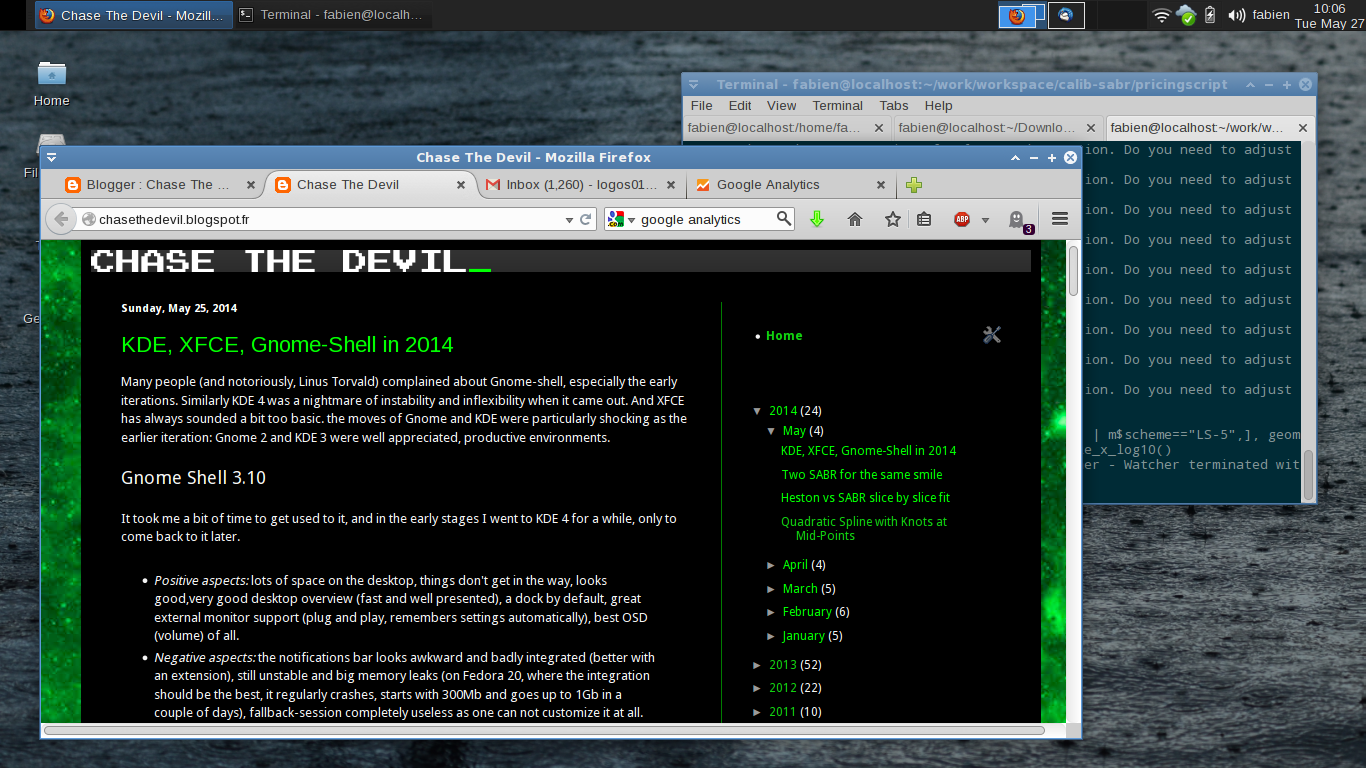
While playing around with differential evolution to calibrate SABR, I noticed that sometimes, several set of parameters can lead to a very similar smile, usually the good one is for relatively low vol of vol and the bad one is for relatively high vol of vol. I first looked for errors in my implementation, but it’s a real phenomenon.
I used the normal implied volatility formula with beta=1, then converted it to lognormal (Black) volatility. While it might not be a great idea to rely on the normal formula with beta=1, I noticed the same phenomenon with the arbitrage free PDE density approach, especially for long maturities. Interestingly, I did not notice such behavior before with other stochastic volatility models like Heston or Schobel-Zhu: I suspect it has to do with the approximations rather than with the true behavior of SABR.
Differential evolution is surprisingly good at finding the global minimum without much initial knowledge, however when there are close fits like this it can be more problematic, usually this requires pushing the population size up. I find that differential evolution is a neat way to test the robustness (as well as performance) of different SABR algorithms as it will try many crazy sets.
In practice, for real world calibration, there is not much use of differential evolution to calibrate SABR as it is relatively simple to find a good initial guess.
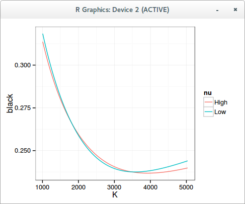
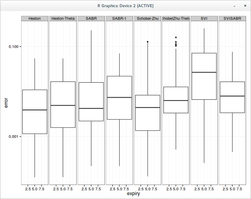
Some people use Heston to fit one slice of a volatility surface. In this case, some parameters are clearly redundant. Still, I was wondering how it fared against SABR, which is always used to fit a slice. And what about Schobel-Zhu?
Aggregated error in fit per slice on 10 surfaces
With Heston, the calibration is actually slightly better with kappa=0, that is, without mean reversion, because the global optimization is easier and the mean reversion is fully redundant. It’s still quite remarkable that 3 parameters result in a fit as good as 5 parameters.
This is however not the case for Schobel-Zhu, where each “redundant parameter” seem to make a slight difference in the quality of calibration. kappa = 0 deteriorate a little bit the fit (the mean error is clearly higher), and theta near 0 (so calibrating 4 parameters) is also a little worse (although better than kappa = 0). Also interestingly, the five parameters Schobel-Zhu fit is slightly better than Heston, but not so when one reduce the number of free parameters.
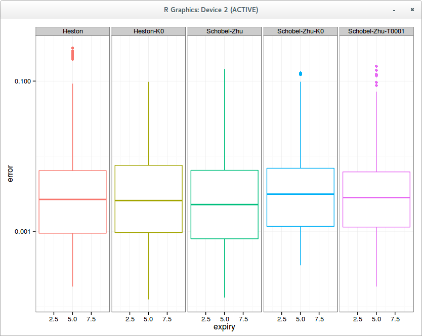
So what about Heston vs SABR. It is interesting to consider the case of general Beta and Beta=1: it turns out that as confirmed for equities, beta=1 is actually a better choice.
Aggregated error in fit per slice on 10 surfaces
Overall on my 10 surfaces composed each of around 10 slices, an admittedly small sample, Heston (without mean-reversion) fit is a little bit better than SABR. Also the SVI-SABR idea from Gatheral is not great: the fit is clearly worse than SABR with Beta=1 and even worse than a simple quadratic.
Of course the best overall fit is achieved with the classic SVI, because it has 6 parameters while the others have only 3.
All the calibrations so far were done slice by slice independently, using levenberg marquardt on an initial guess found by differential evolution. Some people advocate for speed or stability of parameters reasons the idea of calibrating each slice using the previous slice as initial guess with a local optimizer like levenberg marquardt, in a bootstrapping fashion.
The results can be quite different, especially for SVI, which then becomes the worst, even worse than SVI-SABR, which is actually a subset of SVI with fewer parameters. How can this be?
This is because as the number of parameters increases, the first slices optimizations have a disproportionate influence, and finding the real minimum is much more difficult, even with differential evolution for the first slice. It’s easy to picture that you’ll have much more chances to get stuck in some local minimum. It’s interesting to note that the real stochastic volatility models are actually better behaved in this regard, but I am not so sure that this kind of calibration is such a great idea in general.
In practice, the SVI parameters fitted independently evolve in a given surface on each slice in a smooth manner, mostly monotonically. It’s just that to go from one set on one slice to the other on the next slice, you might have to do something more than a local optimization.
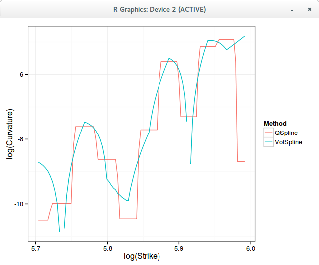
I wondered at the time what a quadratic spline would look like on this problem, as it should be very close in theory, except that we can ensure that it is C1, a condition for a good looking implied volatility.
For a while, I did not find any references around splines where knots are in between two interpolation points and derived my own formula. And then I lost the paper, but out of curiosity, I looked at the excellent De Boor book “A Practical Guide to Splines” and found that there was actually a chapter around this: quadratic splines with knots at mid-points. Interestingly, it turns out that a quadratic spline on standard knots is not always well defined, which is why, if one does quadratic splines, the knots need to be moved.The papers from this era are quite rudimentary in their presentation (the book is much better). I found the paper from Demko 1977 “Interpolation by Quadratic Splines” quite usable for coding. I adjusted the boundaries to make the first and last quadratic fit the first two/last two strikes (adding a first strike at 0 and a large last strike if necessary) and spend countless time worrying about indices. The result on a simple classic example is interesting.
On the non monotonic discrete density data of my earlier blog entry, this gives:
QSpline is the quadratic spline
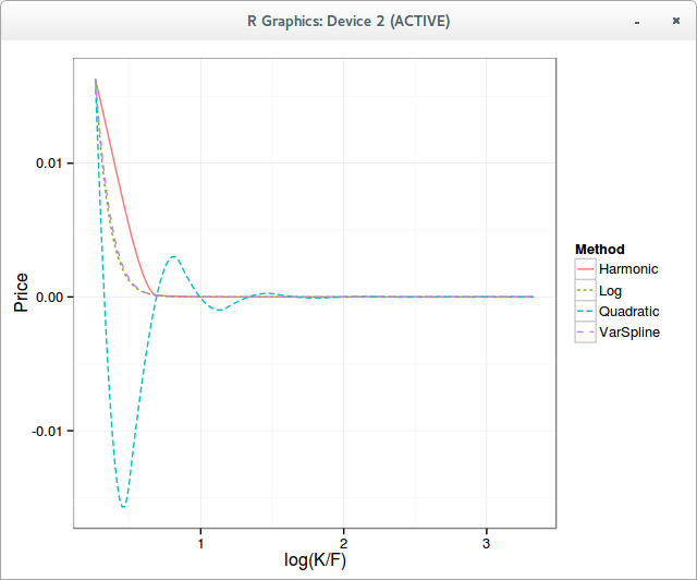
Unfortunately, interpolating small prices with such a spline results in a highly oscillating interpolation: this is the Gibbs phenomenon for splines. We need to loose strict C1 continuity for practical applications, and use a first derivative approximation instead, very much like the Harmonic cubic spline.
On Jaeckel data, the quadratic spline on prices is highly oscillating
I am going to write a little about my experience and conclusions so far around interviewing a candidate for a software developer position or for a quant position, but it should be quite general.
At first, I used to ask interview questions I liked when I was myself a candidate. On the technical side, it would stuff like:
which design patterns do you know?
what’s your opinion on design patterns?<
what’s a virtual method?
any interesting algorithm you like?
which libraries did you use?
For a quant type I’d ask more specific questions:
what’s a Brownian motion?<
what’s the Stratanovitch integral?
why do we use the Ito integral in finance?<
questions on numerical methods: Monte-Carlo and finite differences.
questions on financial details.
I found the approach mostly frustrating: very few people would give interesting (or even good) answers, because most people are not that well prepared for the interview. The exception goes to the academic kind of guy, who usually gives excellent answers, sometimes so good that you feel dumb asking those questions.
People who don’t give good answers could actually be good coworkers. When I was junior, I was particularly bad at job interviews. I did not necessarily know object orienting concepts that well, even if I started programming at an early age. After a few years, I did not know database theory well either because I had experience only with simple queries, having mostly worked on other stuff. A failed interview made me look more closely at the subject, and it turns out that you can sound like an expert after reading only 1 relatively short book (and the theory is actually quite interesting). I went later to the extreme of complex queries, and then realized why ORMs are truely important. Similarly when I first interviewed for the “finance” industry, I sounded very dumb, barely knowing what options were. It’s natural to make mistakes, and to not know much. I learnt all that through various mentor coworkers who indirectly encouraged me with their enthusiasm to read the right stuff. What’s valuable is the ability to learn, and maybe, when you are very experienced, your past experiences (which might not match at all the interviewer knowledge).
Similarly, I sometimes appeared extremely good to interviewers, because it turned out I had practiced similar tests as their own out of curiosity not much time before the interview.
There is also a nasty aspect on asking precise pre-formatted technical questions, you will tend to think that everybody is dumb because they can’t answer those basic questions you know so well, turning you into an arrogant asshole.
I also tried asking probability puzzles (requiring only basic maths knowledge). This gave even less clues towards the candidates in general, except for the exceptional one, where, again you feel a bit dumb for asking those.
In the end, I noticed that the most interesting part of the interview was to discuss a subject the candidate knew well, with the idea of trying to extract knowledge from the candidate, to learn something from him.
I believe this is might be what the interview should only be about. Furthermore, you don’t feel like you are losing your time with such an approach.
I am currently reading the book “Nonlinear Option Pricing” by J. Guyon and P. Henry-Labordère. It’s quite interesting even if the first third is quite theoretical. For example they describe how to solve some not well defined non-linear parabolic PDE by relying on the parabolic envelope. They also explain why most problems lead to parabolic PDEs in finance.
The rest is a bit more practical. I stumbled upon an good remark regarding Longstaff-Schwartz: the algorithm as Longstaff and Schwarz describe it does not necessary lead to a low-biased estimate as they use future information (the paths they regress on) in the Monte-Carlo estimate. It was actually a subject of discussion with colleagues, and I analyzed the numerical impact in a simple use case in http://papers.ssrn.com/abstract=2262259 In short: it’s actually more precise to include the path, even if the estimate is not purely low biased anymore, but the bias is really small in practice.
On the same subject I was a bit surprised that a recent paper on American Monte-Carlo regressed systematically on all paths instead of just a subset. One interesting part of the paper is a way to do successive regressions on different blocks of paths.
Those details are rarely discussed in papers and books. It was comforting to see that I am not alone to wonder about all this.
There is a relatively new JVM based language, Xtend. Their homepage says “JAVA 10, TODAY!”, so I thought I would give it a try, I was especially interested in operator overloading support, and the fact that it compiles to Java code, not Java byte code.
Unfortunately, after 5 minutes with it, and pasting some non Java code in an xtend file, Eclipse hangs forever, even on restart. After creating another workspace, just to trash the new workspace a similar way. This is quite incredible for a nearly 2 years old project, on eclipse.org.
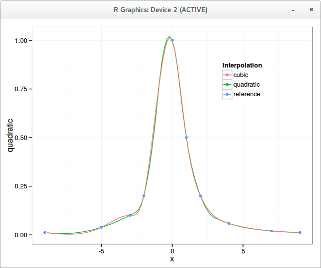
In reality, the problem is much simpler in the Bachelier/Normal model. A very basic analysis of Bachelier formula shows that the problem can be reduced to a single variable, as Choi et al explain in their paper. So the problem is not really one of solving, but one of approximating (the inverse of) a function.
The first step to build that function is to actually have a highly accurate slow solver as reference. This is quite easy, I just started with Choi formula and used Halley's method to refine. In reality, Halley's method is already a bit overkill on this problem: it works impressively well, 1 iteration is enough to have an insane level of accuracy, only noticeable when one works in high precision arithmetic (for example 50 digits). For double precision, Newton's method would actually be enough - I initially thought that my Halley's implementation did not work as it produced the exact same output as Newton in double precision. Li proposes the use of the SOR method, which for this exercise, behaves very much like Newton's method.
I then followed the logic from Choi et al, but working directly with in-the-money call options instead of straddles. Straddles sound neat at first (hides that we work in-the-money), but it's actually useless for the algorithm. Choi et al. ignore half of the straddle range when they use their eta transform in the paper. One other change is the mapping itself, I found a better mapping for the call options (but not that far of Choi initial idea). Finally, because I am lazy, I did not go to the pain of finding a good rational fraction approximation along with the square root problem they describe, I just tried a Chebyshev polynomial.
Unfortunately, a single Chebyshev polynomial does not work well: even with a very large (1000) degree it's not very precise, so much that I thought that my transform was garbage. I had noticed by mistake, that on another part (negative) of the interval, the Chebyshev polynomial worked actually very well to approximate something related to the volatility of another option. Suddendly came to me the idea of, like Johnson does in his Faddeeva package, using N Chebyshev polynomials on N small intervals. This is like the big heavy hammer for which everything looks like nails, but it's actually very fast to evaluate as the degree of each polynomial can then be low (7), plus a table lookup (could be coded as switch statements if one really cares about such details). The slowest part is actually the call to the log function.
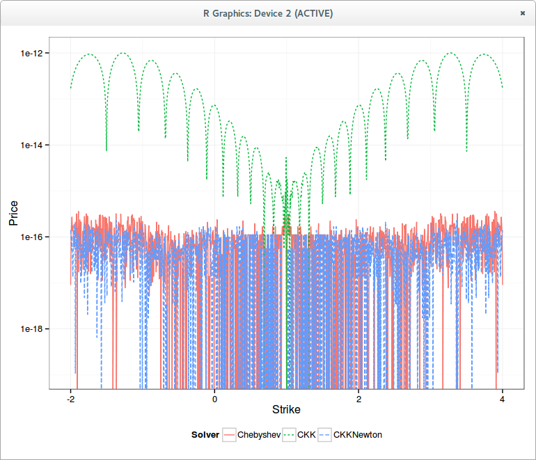
The final bit is the use of a Taylor approximation for my -u/log(1-u) transform as it is not all that accurate in double precision when u is near 0. And that produces the following graph
It is interesting to note that "solving" the b.p. vol is 10x faster than solving the Black vol.
The calibration of a stochastic volatility model or a volatility surface parameterization (like SVI) involves minimizing the model options volatilities against market options volatilities. Often, the model computes an option price, not an implied volatility. It is therefore useful to have a fast way to invert that option price to get back the implied volatility that corresponds to it. Furthermore during the calibration procedure, the model option price can vary widely: it is convenient to have a robust implied volatility solver.
Another more basic use of implied volatility solvers, is for the computation of Black-Scholes greeks for a given market option price.
A few years ago, P. Jaeckel produced a much better algorithm than a simple Newton or Brent solver, in his paper By Implication. There is also a much simpler algorithm from Li, based on SOR and a good initial guess for SOR, which I found to be actually quite robust and fast. Now P. Jaeckel has a newer algorithm, faster and more accurate, close to double accuracy.
I have tested those on 1 million options of random volatility (between 0.001 and 3), random strikes (N deviations with a cap at 1M) for a few expiries.In terms of performance, the results are independent of expiries, but in terms of accuracy, the new Jaeckel algorithm is particularly more accurate for the long-term options (5y and 15y).
Algorithm
Expiry
Vol RMSE
Price RMSE
Time
Jaeckel2014
5y
3.8E-16
2.1E-16
1.8s
Jaeckel2006
5y
1.3E-10
1.1E-10
3.0s
Jaeckel2014
15y
2.0E-12
2.4E-16
1.8s
Jaeckel2006
15y
1.5E-7
8.0E-11
2.7s
The maximum error from Jaeckel2006 is around 1e-8, while the one from Jaeckel2014 is 2e-15 (for very large unrealistic strike)
As a comparison, the simpler Li SOR-TS algorithm follows the given price accuracy independently of the expiry; I have tested with 1E-12. The error in implied volatility will be slightly higher: different close vols can give the same price due to the maximum achievable accuracy of the Black-Scholes formula with double numbers, even with a good cumulative normal distribution implementation. Its performance is however dependent on the number of deviations considered: closer to ATM means faster for Li algorithm.<
Algorithm
Expiry
Deviation
Vol RMSE
Price RMSE
Time
Jaeckel2014
1y
5
4.2E-16
2.0E-17
1.8s
LiSORTS
1y
5
8.5E-9
1.9E-13
2.1s
Jaeckel2014
1y
3
3.1E-16
5.9E-17
1.7s
LiSORTS
1y
3
4.3E-12
1.6E-13
1.3s
Actually, I have cheated in my Li SOR-TS implementation: I have reused the idea from P. Jaeckel to compute the Black-Scholes price with erfc_x (unscaled erfc) instead of erfc. This simple change divides the number of exp calls by 2. Without this trick, for 5 deviations, SOR-TS took 3.6s (almost twice the time).
I would not be surprised if this was the main performance improvement between the two Jaeckels.