Implying the Probability Density from Market Option Prices
In the previous post, I showed a plot of the probability implied from SPW options before and after the big volatility change of last week. I created it from a least squares spline fit of the market mid implied volatilities (weighted by the inverse of the bid-ask spread). While it looks reasonable, the underlying technique is not very robust. It is particularly sensitive to the number of options strikes used as spline nodes.
Below I vary the number of nodes, by considering nodes at every N market strikes, for different values of N.
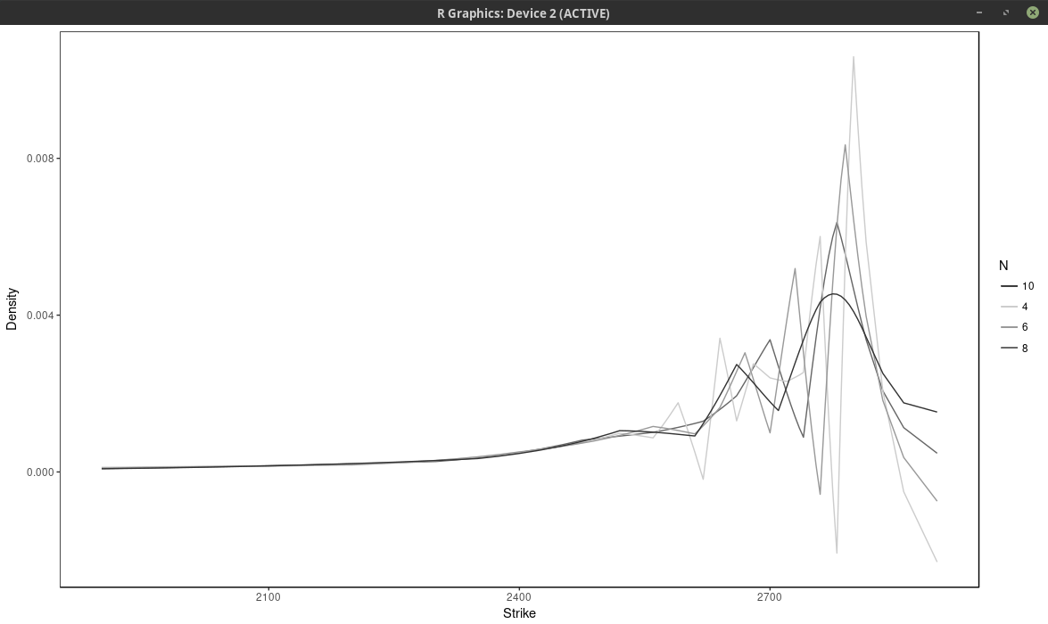
probability density of the SPX implied from 1-month SPW options with nodes located at every N market strike, for different values of N. Least squares spline approach
With \(N \leq 6\), the density has large wiggles, that go into the negative half-plane. As expected, a large N produces a flatter and smoother density. It is not obvious which value of N is the most appropriate.
Another technique is to fit directly a weighted sum of Gaussian densities, of fixed standard deviation, where the weights are calibrated to the market option prices. This is described in various papers and books from Wystup such as this one. He calls it the kernel slice approach. If we impose that the weights are positive and sum to one, the resulting model density will integrate to one and be positive.
It turns out that the price of a Vanilla option under this model is just the sum of vanilla options prices under the Bachelier model with shifted forwards (each “optionlet” forward corresponds to a peak on the market strike axis). So it is easy and fast to compute. But more importantly, the problem of finding the weights is linear. In deed, the typical measure to minimize is: $$ \sum_{i=0}^{n} w_i^2 \left( C_i^M -\sum_{j=1}^m Q_j C_j^B(K_i) \right)^2 $$ where \( w_i \) is a market weight related to the bid-ask spread, \( C_i^M \) is the market option price with strike \( K_i \), \( C_j^B(K_i) \) is the j-th Bachelier optionlet price with strike \( K_i \) and \( Q_j \) is the optionlet weight we want to optimize.
The minimum is located where the gradient is zero. $$ \sum_{i=0}^{n} 2 w_i^2 C_k^B(K_i) \left( C_i^M -\sum_{j=1}^m Q_j C_j^B(K_i) \right) = 0 \text{ for } k=1,…,m $$ It is a linear and can be rewritten in term of matrices as \(A Q = B\) but we have the additional constraints $$ Q_j \geq 0 $$ $$ \sum_j Q_j = 1 $$
The last constraint can be easily added with a Lagrange multiplier (or manually by elimination). The positivity constraint requires more work. As the problem is convex, the solution must lie either inside or on a boundary. So we need to explore each case where \(Q_k = 0\) for one or several k in 1,…m. In total we have \(2^{m-1}-1\) subsets to explore.
How to list all the subsets of \( \{1,…,m\} \)? It turns out it is very easy by using a bijection of each subset with the binary representation of \( {0,…,2^m} \). We then just need to increment a counter for 1 to \( 2^m \) and transform the binary representation to our original set elements. Each element of the subset corresponds to a 1 in the binary representation.
Now this works well if m is not too large as we need to solve \(2^{m-1}-1\) linear systems. I actually found amazing, it took only a few minutes for m as high as 26 without any particular optimization. For m larger we need to be more clever. One possibility is to solve the unconstrained problem, and put all the negative quantities to 0 in the result, then solve again this new problem on those boundaries and repeat until we find a solution. This simple algorithm works often well, but not always. There exists specialized algorithms that are much better and nearly as fast. Unfortunately I was too lazy to code them. So I improvised on the Simplex. The problem can be transformed into something solvable by the Simplex algorithm. We maximize the function \( -\sum_j Z_j \) with the constraints $$ A Q - I Z = B $$ $$ Q_j \geq 0 $$ $$ Z_j \geq 0 $$ where I is the identity matrix. The additonal Z variables are slack variables, just here to help transform the problem. This is a trick I found on a researchgate forum. The two problems are not fully equivalent, but they are close enough that the Simplex solution is quite good.
With the spline, we minimize directly bid-ask weighted volatilities. With the kernel slice approach, the problem is linear only terms of call prices. We could use a non-linear solver with a good initial guess. Instead, I prefer to transform the weights so that the optimal solution on weighted prices is similar to the optimal solution on weighted volatilities. For this, we can just compare the gradients of the two problems: $$ \sum_{i=0}^{n} 2 {w}_i^2 \frac{\partial C}{\partial \xi}(\xi, K_i) \left( C_i^M - C(\xi, K_i) \right) $$ with $$ \sum_{i=0}^{n} 2 {w^\sigma_i}^2\frac{\partial \sigma}{\partial \xi}(\xi, K_i) \left( \sigma_i^M - \sigma(\xi, K_i)\right) $$ As we know that $$ \frac{\partial C}{\partial \xi} = \frac{\partial \sigma}{\partial \xi} \frac{\partial C}{\partial \sigma} $$ we approximate \( \frac{\partial C}{\partial \sigma} \) by the market Black-Scholes Vega and \( \left( C_i^M - C(\xi, K_i) \right) \) by \( \frac{\partial C}{\partial \xi} (\xi_{opt}-\xi) \), \( \left( \sigma_i^M - \sigma(\xi, K_i) \right) \) by \( \frac{\partial \sigma}{\partial \xi} (\xi_{opt}-\xi) \) to obtain $$ {w}_i \approx \frac{1}{ \frac{\partial C_i^M}{\partial \sigma_i^M} } {w^\sigma_i} $$
Now it turns out that the kernel slice approach is quite sensitive to the choice of nodes (strikes), but not as much as to the choice of number of nodes. Below is the same plot as with the spline approach, that is we choose every N market strike as node. For N=4, the density is composed of the sum of m/4 Gaussian densities. We optimized the kernel bandwidth (here the standard deviation of each Gaussian density), and found that it was relatively insensitive to the number of nodes, in our case around 33.0 (in general it is expected to be about three times the order the distance between two consecutive strikes, which is 5 to 10 in our case), a smaller value will translate to narrower peaks.
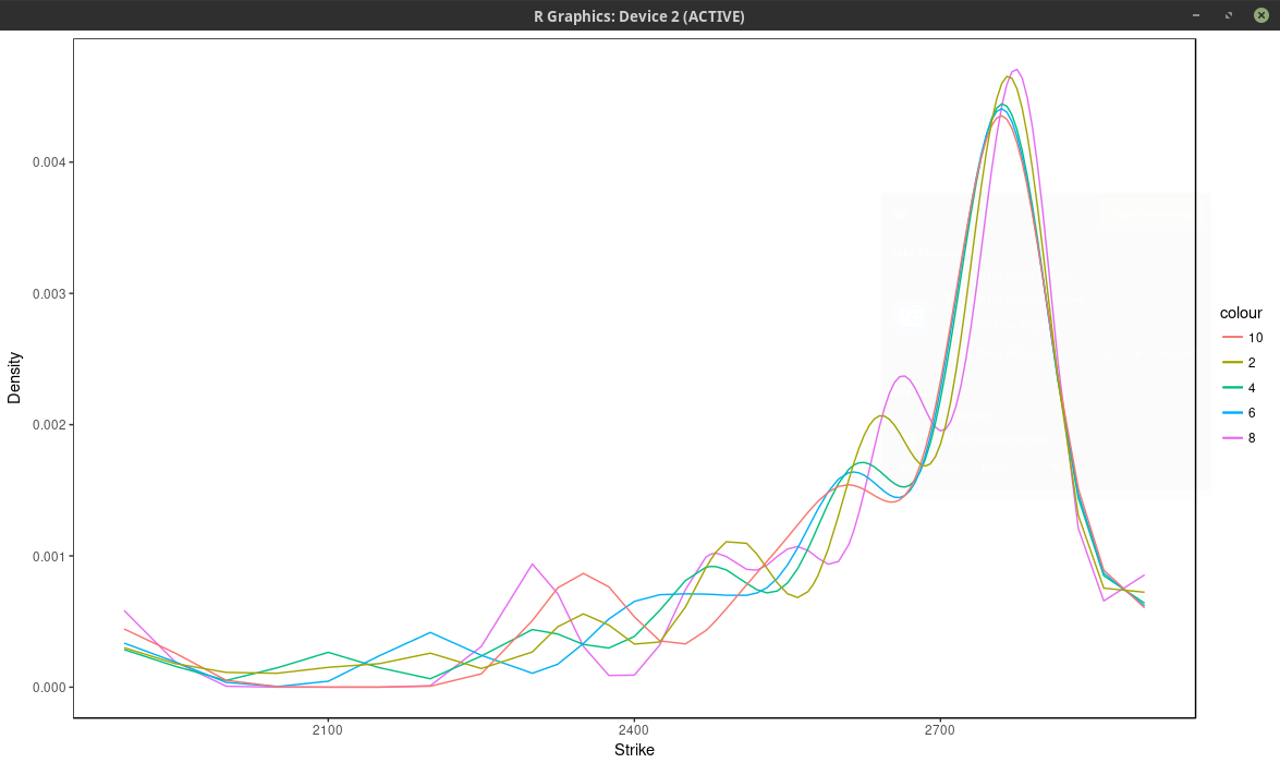
probability density of the SPX implied from 1-month SPW options with nodes located at every N market strike, for different values of N. Kernel slice approach.
Even if we consider here more than 37 nodes (m=75 market strikes), the optimal solution actually use only 13 nodes, as all the other nodes have a calibrated weight of 0. The fit can be much better by adding nodes at f * 0.5, f * 0.8, f * 0.85, f * 0.9, f * 0.95, f * 0.98, f, f * 1.02, f * 1.05, f * 1.1, f * 1.2, f * 1.5, where f is the forward price, even though the optimal solution will only use 13 nodes again. We can see this by looking at the implied volatility.
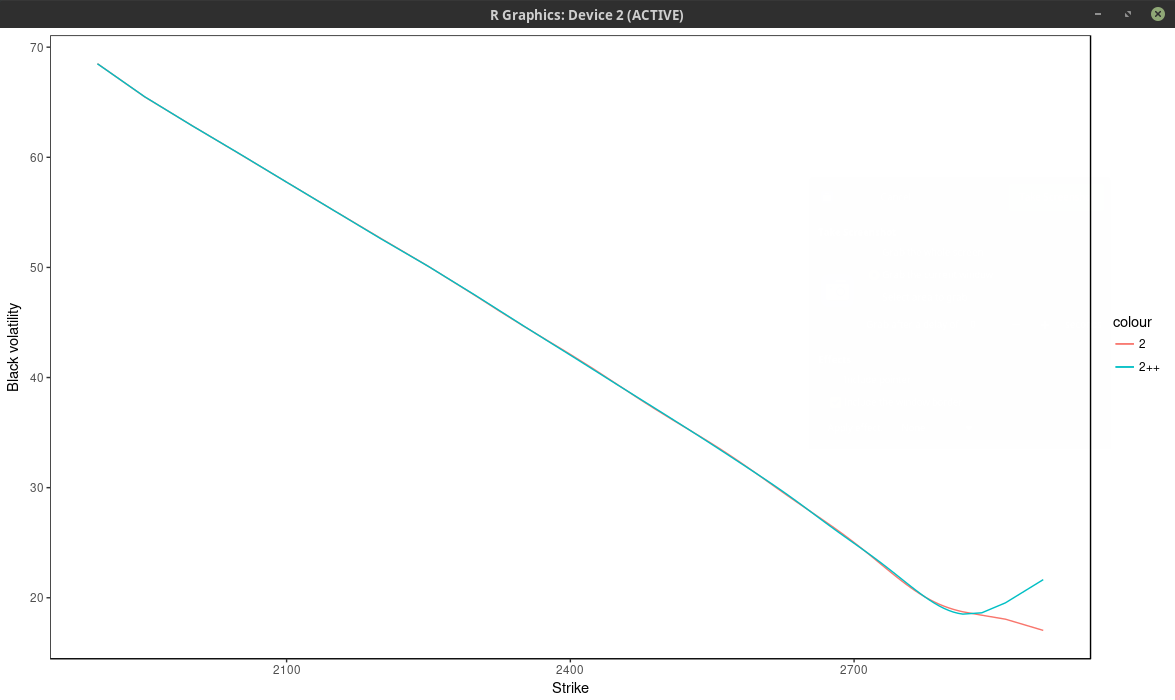
implied volatility of the SPX implied from 1-month SPW options with nodes located at every 2 market strike.
Using only the market nodes does not allow to capture right wing of the smile. The density is quite different between the two.
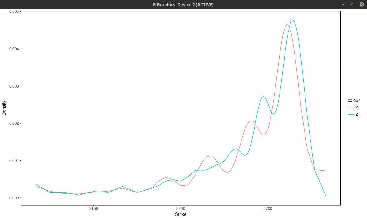
density of the SPX implied from 1-month SPW options with nodes located at every 2 market strike.
I found (surprisingly) that even those specific nodes by themselves (without any market strike) work better than using all market strikes (without those nodes), but then we impose where the peaks will be located eventually.
It is interesting to compare the graph with the one before the volatility jump:
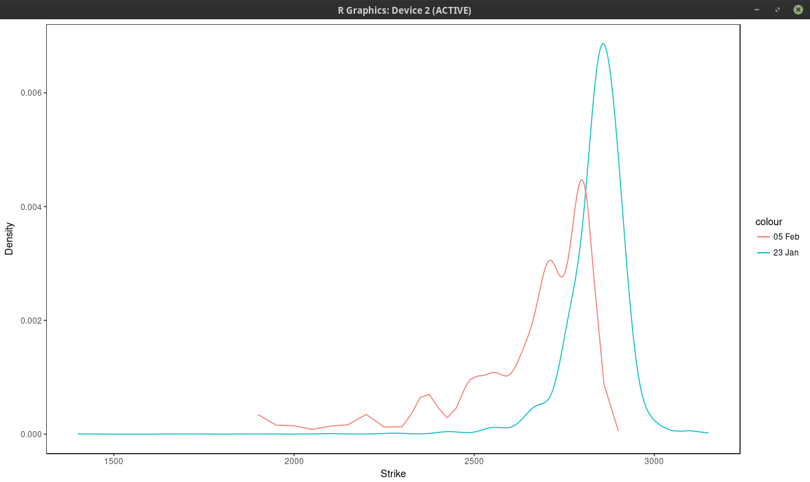
density of the SPX implied from 1-month SPW options with nodes located at every 2 market strike.
So in calm markets, the density is much smoother and has really only one main mode/peak.
It is possible to use other kernels than the Gaussian kernel. The problem to solve would be exactly the same. It is not clear what would be the advantages of another kernel, except, possibly, speed to solve the linear system in O(n) operations for a compact kernel spanning at most 3 nodes (which would translate to a tridiagonal system).