I am on holiday today. Unfortunately I am still thinking about work-related matters, and out of curiosity, wanted to do a little experiment. I know it is not very good to spend free time on work related stuff: there is no reward for it, and there is so much more to life. Hopefully it will be over after this post.
Around 2 years ago, I saw a presentation from Andreasen and Huge about how they were able to price/calibrate SABR by a one-step finite difference technique. At that time, I did not understand much their idea. My mind was too focused on more classical finite differences techniques and not enough on the big picture in their idea. Their idea is quite general and can be applied to much more than SABR.
Recently there has been some talk and development going on where I work about SABR (a popular way to interpolate the option implied volatility surface for interest rate derivatives), especially regarding the implied volatility wings at low strike, and sometimes on how to price in a negative rates environment. There are actually quite a bit of research papers around this. I am not really working on that part so I just mostly listened. Then a former coworker suggested that the Andreasen Huge method was actually what banks seemed to choose in practice. A few weeks later, the Thalesians (a group for people interested in quantitative finance) announced a presentation by Hagan (one of the inventor of SABR) about a technique that sounded very much like Andreasen-Huge to deal with the initial SABR issues in low rates.
As the people working on this did not investigate Andreasen-Huge technique, I somehow felt that I had to and that maybe, this time, I would be able to grasp their idea.
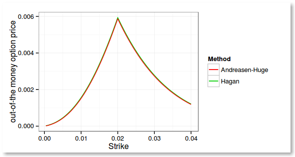
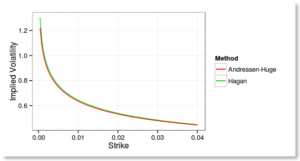
It took me just a few hours to have meaningful results. Here is the price of out of the money vanilla options using alpha = 0.0758194, nu = 0.1, beta = 0.5, rho = -0.1, forward = 0.02, and a maturity of 2 years.
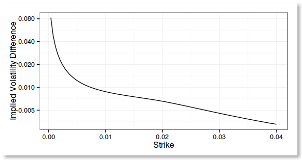
I did not have in my home library a way to find the implied volatility for a given price. I knew of 2 existing methods, Jaeckel "By Implication", and Li rational functions approach. I discovered that Li wrote a new paper on the subject where he uses a SOR method to find the implied volatility and claims it's very accurate, very fast and very robust. Furthermore, the same idea can be applied to normal implied volatility. What attracted me to it is the simplicity of the underlying algorithm. Jaeckel's way is a nice way to do Newton-Raphson, but there seems to be so many things to "prepare" to make it work in most cases, that I felt it would be too much work for my experiment. It took me a few more hours to code Li SOR solvers, but it worked amazingly well for my experiment.
At first I had an error in my boundary condition and had no so good results especially with a long maturity. The traps with Andreasen-Huge technique are very much the same as with classical finite differences: be careful to place the strike on the grid (eventually smooth it), and have good boundaries.
Van Haastrecht, Lord and Pelsser present an effective way to price derivatives by Monte-Carlo under the Schobel-Zhu model (as well as under the Schobel-Zhu-Hull-White model). It's quite similar to Andersen QE scheme for Heston in spirit.
In their paper they evolve the (log) asset process together with the volatility process, using the same discretization times. A while ago, when looking at Joshi and Chan large steps for Heston, I noticed that, inspired by Broadie-Kaya exact Heston scheme, they present the idea to evolve the variance process using small steps and the asset process using large steps (depending on the payoff) using the integrated variance value computed by small steps. The asset steps correspond to payoff evaluation dates At that time I had applied this idea to Andersen QE scheme and it worked reasonably well.
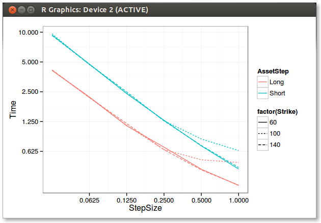
So I tried to apply the same logic to Schobel Zhu, and my first tests show that it works too. Interestingly, the speed gain is about 2x. Here are the results for a vanilla call option of different strikes.
Similar Error between long and short asset steps
Long steps take around 1/2 the time to compute
I would have expected the difference in performance to increase when the step size is decreasing, but it's not the case on my computer.
It's not truly large steps like Joshi and Chan do in their integrated double gamma scheme as the variance is still discretized in relatively small steps in my case, but it seems like a good, relatively simple optimization. A while ago, I did also implement the full Joshi and Chan scheme, but it's really interesting if one is always looking for long steps: it is horribly slow when the step size is small, which might occur for many exotic payoffs, while Andersen QE scheme perform almost as well as log-Euler in terms of computational cost.
Where I work, there used to be quite a bit of a confusion on which rates one should use as input to a Local Volatility Monte-Carlo simulation.
In particular there is a paper in the Journal of Computation Finance by Andersen and Ratcliffe “The Equity Option Volatility Smile: a Finite Difference Approach” which explains one should use specially tailored rates for the finite difference scheme in order to reproduce exact Bond price and exact Forward contract prices
Code has been updated and roll-backed, people have complained around it. But nobody really made the effort to simply write clearly what’s going on, or even write a unit test around it. So it was just FUD, until this paper.
In short, for log-Euler, one can use the intuitive forward drift rate: r1t1-r0t0 (ratio of discount factors), but for Euler, one need to use a less intuitive forward drift rate to reproduce a nearly exact forward price.
I have been wondering if there was any better alternative than the standard Sobol (+ Brownian Bridge) quasi random sequence generator for the Monte Carlo simulations of finance derivatives.
Here is what I found:
Scrambled Sobol. The idea is to rerandomize the quasi random numbers slightly. It can provide better uniformity properties and allows for a real estimate of the standard error. There are many ways to do that. The simple Cranley Patterson rotation consisting in adding a pseudo random number modulo 1, Owen scrambling (permutations of the digits) and simplifications of it to achieve a reasonable speed. This is all very well described in Owen Quasi Monte Carlo document
Lattice rules. It is another form of quasi random sequences, which so far was not very well adapted to finance problems. A presentation from Giles & Kuo look like it's changing.
Fast PCA. An alternative to Brownian Bridge is the standard PCA. The problem with PCA is the performance in O(n^2). A possible speedup is possible in the case of a equidistant time steps. This paper shows it can be generalized. But the data in it shows it is only advantageous for more than 1024 steps - not so interesting in Finance.
Recently, that I completed a project that I had initially estimated to around 2 months, in nearly 4 hours. This morning I fixed the few remaining bugs. I looked at the clock, surprised it was still so early and I still had so many hours left in the day.
Now I have more time to polish the details and go beyond the initial goal (I think this scares my manager a bit), but I could (and I believe some people do this often) stop now and all the management would be satisfied.
What’s interesting is that everybody bought the 2 months estimate without questions (I almost even believed it myself). This reminded me of my productivity zero post.
Glasserman and Yu (GY) give a relatively simple algorithm to compute lower and upper bounds of a the price of a Bermudan Option through Monte-Carlo.
I always thought it was very computer intensive to produce an upper bound, and that the standard Longstaff Schwartz algorithm was quite precise already. GY algorithm is not much slower than the Longstaff-Schwartz algorithm, but what's a bit tricky is the choice of basis functions: they have to be Martingales. This is the detail I overlooked at first and I, then, could not understand why my results were so bad. I looked for a coding mistake for several hours before I figured out that my basis functions were not Martingales. Still it is possible to find good Martingales for the simple Bermudan Put option case and GY actually propose some in another paper.
Here are some preliminary results where I compare the random number generator influence and the different methods. I include results for GY using In-the-money paths only for the regression (-In suffix) or all (no suffix).
value using 16k training path and Sobol - GY-Low-In is very close to LS.
error using 16k training path - a high number of simulations not that useful
error using 1m simulation paths - GY basis functions require less training than LS
One can see the the upper bound is not that precise compared to the lower bound estimate, and that using only in the money paths makes a big difference. GY regression is good with only 1k paths, LS requires 10x more.
Surprisingly, I noticed that the Brownian bridge variance reduction applied to Sobol was increasing the GY low estimate, so as to make it sometimes slightly higher than Longstaff-Schwartz price.
Already the name United Nations should be suspicious, but now they are shown to have spread Cholera to Haiti, as if the country did not have enough suffering. They have a nice building in New-York, and used to have a popular representative, but unfortunately, for poor countries, they never really achieved much. In Haiti, there were many stories of rapes and corruption by U.N. members more than 10 years ago. The movie The Whistleblower suggests it was the same in the Balkans. I am sure it did not change much since.
Dropbox worked well, but the company decided to blacklist it. I suppose some people abused it. While looking for an alternative, I found Ubuntu One. It’s funny I never tried it before even though I use Ubuntu. I did not think it was a dropbox replacement, but it is. And you get 5GB instead of Dropbox 2GB limit, which is enough for me (I was a bit above the 2GB limit). It works well under Linux but as well on Android and there is an iOS app I have not yet tried. It also works on Windows and Mac.
In the book Monte Carlo Methods in Financial Engineering, Glasserman explains that if one reuses the paths used in the optimization procedure for the parameters of the exercise boundary (in this case the result of the regression in Longstaff-Schwartz method) to compute the Monte-Carlo mean value, we will introduce a bias: the estimate will be biased high because it will include knowledge about future paths.
However Longstaff and Schwartz seem to just reuse the paths in their paper, and Glasserman himself, when presenting Longstaff-Schwartz method later in the book just use the same paths for the regression and to compute the Monte-Carlo mean value.
How large is this bias? What is the correct methodology?
I have tried with Sobol quasi random numbers to evaluate that bias on a simple Bermudan put option of maturity 180 days, exercisable at 30 days, 60 days, 120 days and 180 days using a Black Scholes volatility of 20% and a dividend yield of 6%. As a reference I use a finite difference solver based on TR-BDF2.
I found it particularly difficult to evaluate it: should we use the same number of paths for the 2 methods or should we use the same number of paths for the monte carlo mean computation only? Should we use the same number of paths for regression and for monte carlo mean computation or should the monte carlo mean computation use much more paths?
I have tried those combinations and was able to clearly see the bias only in one case: a large number of paths for the Monte-Carlo mean computation compared to the number of paths used for the regression using a fixed total number of paths of 256*1024+1, and 32*1024+1 paths for the regression.
Those numbers are too good to be a real. If one reduces too much the total number of paths or the number of paths for the regression, the result is not precise enough to see the bias. For example, using 4K paths for the regression leads to 2.83770 vs 2.83767. Using 4K paths for regression and only 16K paths in total leads to 2.8383 vs 2.8387. Using 32K paths for regressions and increasing to 1M paths in total leads to 2.838539 vs 2.838546.
For this example the Longstaff-Schwartz price is biased low, the slight increase due to path reuse is not very visible and most of the time does not deteriorate the overall accuracy. But as a result of reusing the paths, the Longstaff-Schwartz price might be higher than the real value.
In finance, because one often dicretize the log process instead of the direct process for Monte-Carlo simulation, the Math.exp function can be called a lot (millions of times for a simulation) and can be a bottleneck. I have noticed that the simpler Euler discretization was for local volatility Monte-Carlo around 30% faster, because it avoids the use of Math.exp.
Can we improve the speed of exp over the JDK one? At first it would seem that the JDK would just call either the processor exp using an intrinsic function call and that should be difficult to beat. However what if one is ok for a bit lower accuracy? Could a simple Chebyshev polynomial expansion be faster?
Out of curiosity, I tried a Chebyshev polynomial expansion with 10 coefficients stored in a final double array. I computed the coefficient using a precise quadrature (Newton-Cotes) and end up with 1E-9, 1E-10 absolute and relative accuracy on [-1,1].
Here are the results of a simple sum of 10M random numbers:
0.75s for Math.exp sum=1.7182816693332244E7 0.48s for ChebyshevExp sum=1.718281669341388E7 0.40s for FastMath.exp sum=1.7182816693332244E7
So while this simple implementation is actually faster than Math.exp (but only works within [-1,1]), FastMath from Apache commons maths, that relies on a table lookup algorithm is just faster (in addition to being more precise and not limited to [-1,1]).
Of course if I use only 5 coefficients, the speed is better, but the relative error becomes around 1e-4 which is unlikely to be satisfying for a finance application.
0.78s for Math.exp sum=1.7182816693332244E7 0.27s for ChebyshevExp sum=1.718193001875838E7 0.40s for FastMath.exp sum=1.7182816693332244E7