I stumbled upon an unexpected problem: the one touch barrier formula can break down under negative rates. While negative rates can sound fancy, they are actually quite real on some markets. Combined with relatively low volatilities, this makes the standard Black-Scholes one touch barrier formula blow up because somewhere the square root of a negative number is taken.
At first, I had the idea to just floor the number to 0. But then I needed to see if this rough approximation would be acceptable or not. So I relied on a TR-BDF2 discretization of the Black-Scholes PDE, where negative rates are not a problem.
Later, I was convinced that we ought to be able to find a closed form formula for the case of negative rates. I went back to the derivation of the formula, the book from Kwok is quite good on that. The closed form formula just stems from being the solution of an integral of the first passage time density (which is a simpler way to compute the one touch price than the PDE approach). It turns out that, then, the closed form solution to this integral with negative rates is just the same formula with complex numbers (there are actually some simplifications then).
It is a bit uncommon to use the cumulative normal distribution on complex numbers, but the error function on complex numbers is more popular: it's actually even on the wikipedia page of the error function. And it can be computed very quickly with machine precision thanks to the Faddeeva library.
With this simple closed form formula, there is no need anymore for an approximation. I wrote a small paper around this here.
Later a collegue made the remark that it could be interesting to have the bivariate complex normal distribution for the case of partial start one touch options or partial barrier option rebates (not sure if those are common). Unfortunately I could not find any code or paper for this. And after asking Prof. Genz (who found a very elegant and fast algorithm for the bivariate normal distribution), it looks like an open problem.
In this case, it turns out that the Vogt initial guess method (guess via asymptotes and minimum variance) is actually very good as long as one has a good way to lookup the asymptotes (the data is not always convex, while SVI is) and as long as rho is not close to -1, that is for long maturity affine like smiles, where SVI is actually more difficult to calibrate properly due to the over-parameterisation in those cases.
Still after looking at all of this, one has a sense that, even though it works on a wide variety of surfaces, it could break down because of the complexity: are asymptotes ok, is rho close to -1? how close? is ATM better or maximum curvature better? how do we impose boundaries on a and sigma with Levenberg-Marquardt? (truncation should not be too close to the transform, but how far?)
This is where the Quasi-Explicit method from Zeliade is very interesting: it is simpler, not necessarily to code, but the method itself. There are things to take care of (solving at each boundary), but those are mathematically well defined. The only drawback is performance, as it can be around 40 times slower. But then it’s still not that slow.
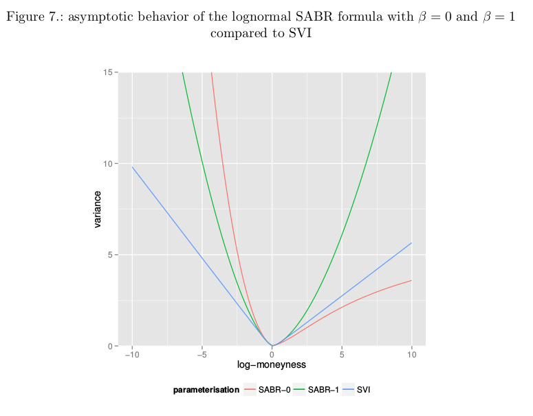
The variance under SVI becomes linear when the log-moneyness is very large in absolute terms. The lognormal SABR formula with beta=0 or beta=1 has a very different behavior. Of course, the theoretical SABR model has actually a different asymptotic behavior.
As an illustration, we calibrate SABR (with two different values of beta) and SVI against the same implied volatility slice and look at the wings behavior.
While the Lee moments formula implies that the variance should be at most linear, something that the SABR formula does not respect. It is in practice not the problem with SABR as the actual Lee boundary: V(x) < 2|x|/T (where V is the square of the implied volatility and x the log-moneyness) is attained for extremely low strikes only with SABR, except maybe for very long maturities.
A related behavior is the fact that the lognormal SABR formula can actually match steeper curvatures at the money than SVI for given asymptotes.
On long maturities equity options, the smile is usually very much like a skew: very little curvature. This usually means that the SVI rho will be very close to -1, in a similar fashion as what can happen for the the correlation parameter of a real stochastic volatility model (Heston, SABR).
In terms of initial guess, I looked at the more usual use cases and showed that matching a parabola at the minimum variance point often leads to a decent initial guess if one has an ok estimate of the wings. We will see here that we can do also something a bit better than just a flat slice at-the-money in the case where rho is close to -1.
In general when the asymptotes lead to rho < -1, it means that we can’t compute b from the asymptotes as there is in reality only one usable asymptote, the other one having a slope of 0 (rho=-1). The right way is to just recompute b by matching the ATM slope (which can be estimated by fitting a parabola at the money). Then we can try to match the ATM curvature, there are two possibilities to simplify the problem: s » m or m » s.
Interestingly, there is some kind of discontinuity at m = 0:
when m = 0, the at-the-money slope is just b*rho.
when m != 0 and m » s, the at-the-money slope is b*(rho-1).
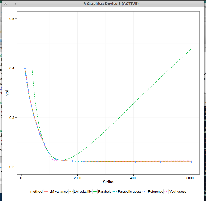
In general it is therefore a bad idea to use m=0 in the initial guess. It appears then that assuming m » s is better. However, in practice, with this choice, the curvature at the money is matched for a tiny m, even though actually the curvature explodes (sigma=5e-4) at m (so very close to the money). This produces this kind of graph:
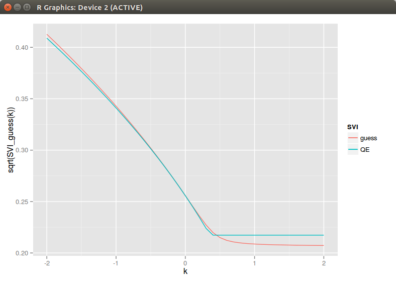
This apparently simple issue is actually a core problem with SVI. Looking back at our slopes but this time in the moneyness coordinate, the slope at m is \(b \rho\) while the slope at the money is \(b(\rho-1)\) if m != 0. If s is small, as the curvature at m is just b/s this means that our there will always be this funny shape if s is small. It seems then that the best we can do is hide it: let m > max(moneyness) and compute the sigma to match the ATM curvature. This leads to the following:
This is all good so far. Unfortunately running a minimizer on it will lead to a solution with a small s. And the bigger picture looks like this (QE is Zeliade Quasi-Explicit, Levenberg-Marquardt would give the same result):
Of course a simple fix is to not let s to be too small, but how do we defined what is too small? I have found that a simple rule is too always ensure that s is increasing with the maturity supposing that we have to fit a surface. This rule has also a very nice side effect that spurious arbitrages will tend to disappear as well. On the figure above, I can bet that there is a big arbitrage at k=m for the QE result.
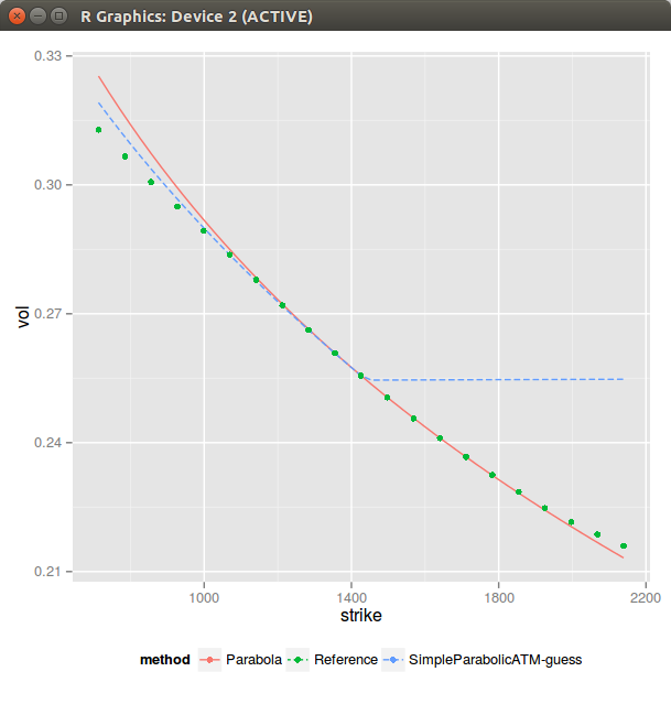
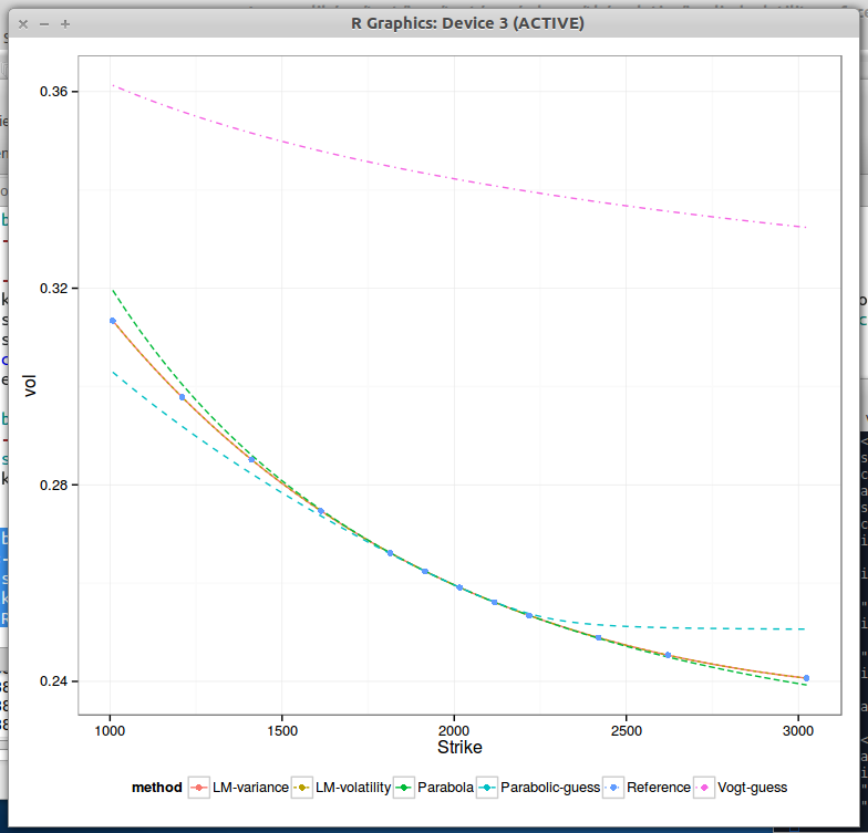
In the previous post, I showed one could extract the SVI parameters from a best fit parabola at-the-money. It seemed to work reasonably well, but I found some real market data where it can be much less satisfying.
Sometimes (actually not so rarely) the ATM slope and curvatures can't be matched given rho and b found through the asymptotes. As a result if I force to just match the curvature and set m=0 (when the slope can't be matched), the simple ATM parabolic guess looks shifted. It can be much worse than this specific example.
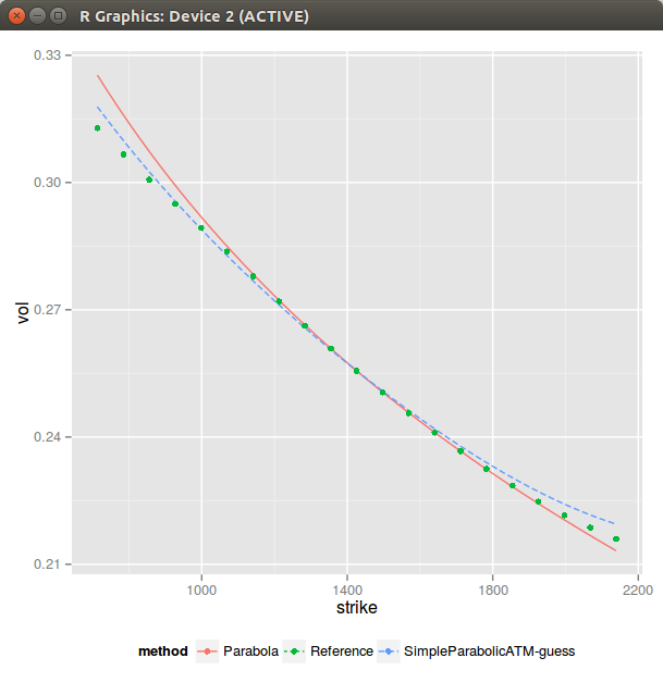
It is then a bit clearer why Vogt looked to match the lowest variance instead of ATM. We can actually also fit a parabola at the lowest variance (MV suffix in the graph) instead of ATM. It seems to fit generally better.
I also tried to estimate the asymptotic slopes more precisely (using the slope of the 5-points parabola at each end), but it seems to not always be an improvement.
However this does not work when rho is close to -1 or 1 as there is then no minimum. Often, matching ATM also does not work when rho is -1 or 1. This specific case, but quite common as well for longer expiries in equities need more thoughts, usually a constant slice is ok, but this is clearly where Zeliade's quasi explicit method shines.
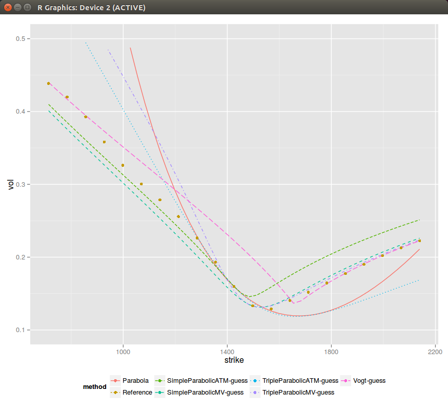
So far it still all looks good, but then looking at medium maturities (1 year), sometimes all initial guesses don't look comforting (although Levenberg-Marquardt minimization still works on those - but one can easily imagine that it can break as well, for example by tweaking slightly the rho/b and look at what happens then).
There is lots of data on this 1 year example. One can clearly see the problem when the slope can not be fitted ATM (SimpleParabolicATM-guess), and even if by chance when it can (TripleParabolicATM-guess), it's not so great. Similarly fitting the lowest variance leads only to a good fit of the right wing and a bad fit everywhere else.
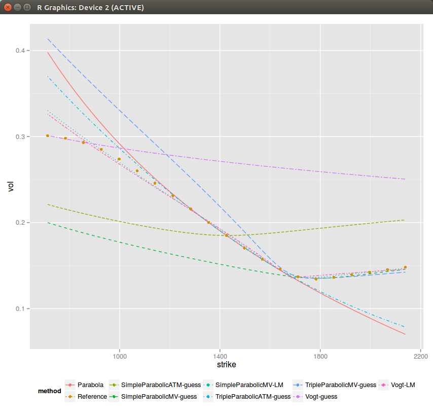
Still, as if by miracle, everything converges to the best fit on this example (again one can find cases where some guesses don't converge to the best fit). I have added some weights +-20% around the money, to ensure that we capture the ATM behavior accurately (otherwise the best fit is funny).
It is interesting to see that if one minimizes the min square sum of variances (what I do in Vogt-LM, it's in theory slightly faster as there is no sqrt function cost) it results in an ugly looking steeper curvature, while if we just minimize the min square sum of volatilities (what I do in SimpleParabolicMV_LM), it looks better.
The SVI formula is: $$w(k) = a + b ( \rho (k-m) + \sqrt{(k-m)^2+ \sigma^2}$$ where k is the log-moneyness, w(k) the implied variance at a given moneyness and a,b,rho,m,sigma the 5 SVI parameters.
A. Vogt described a particularly simple way to find an initial guess to fit SVI to an implied volatility slice a while ago. The idea to compute rho and sigma from the left and right asymptotic slopes. a,m are recovered from the crossing point of the asymptotes and sigma using the minimum variance.
Later, Zeliade has shown a very nice reduction of the problem to 2 variables, while the remaining 3 can be deduced explicitly. The practical side is that constraints are automatically included, the less practical side is the choice of minimizer for the two variables (Nelder-Mead) and of initial guess (a few random points).
Instead, a simple alternative is the following: given b and rho from the asymptotic slopes, one could also just fit a parabola at-the-money, in a similar spirit as the explicit SABR calibration, and recover explicitly a, m and sigma.
To illustrate I take the data from Zeliade, where the input is already some SVI fit to market data.
3M expiry - Zeliade data
4Y expiry, Zeliade data
We clearly see that ATM the fit is better for the parabolic initial guess than for Vogt, but as one goes further away from ATM, Vogt guess seems better.
Compared to SABR, the parabola itself fits decently only very close to ATM. If one computes the higher order Taylor expansion of SVI around k=0, powers of (k/sigma) appear, while sigma is often relatively small especially for short expiries: the fourth derivative will quickly make a difference.
On implied volatilities stemming from a SABR fit of the SP500, here is how the various methods behave:
1M expiry on SABR data
4Y expiry on SABR data
As expected, because SABR (and thus the input implied vol) is much closer to a parabola, the parabolic initial guess is much better than Vogt. The initial guess of Vogt is particularly bad on long expiries, although it will still converge quite quickly to the true minimum with Levenberg-Marquardt.
In practice, I have found the method of Zeliade to be very robust, even if a bit slower than Vogt, while Vogt can sometimes (rarely) be too sensitive to the estimate of the asymptotes.
The parabolic guess method could also be applied to always fit exactly ATM vol, slope and curvature, and calibrate rho, b to gives the best overall fit. It might be an idea for the next blog post.
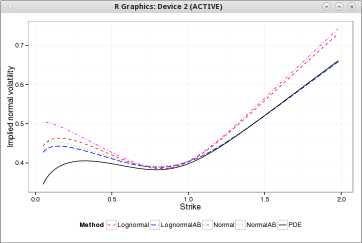
In a talk at the Global Derivatives conference of Amsterdam (2014), Pat Hagan presented some new SABR formulas, supposedly close to the arbitrage free PDE behavior.
I tried to code those from the slides, but somehow that did not work out well on his example, I just had something very close to the good old SABR formulas. I am not 100% sure (only 99%) that it is due to a mistake in my code. Here is what I was looking to reproduce:
Pat Hagan Global Derivatives example
Fortunately, I then found in some thesis the idea of using Andersen & Brotherton-Ratcliffe local volatility expansion. In deed, the arbitrage free PDE from Hagan is equivalent to some Dupire local volatility forward PDE (see http://papers.ssrn.com/abstract=2402001), so Hagan just gave us the local volatility expansion to expand on (the thesis uses Doust, which is not so different in this case).
And then it produces on this global derivatives example the following:
The AB suffix are the new SABR formula. Even though the formulas are different, that looks very much like Hagan's own illustration (with a better scale)!
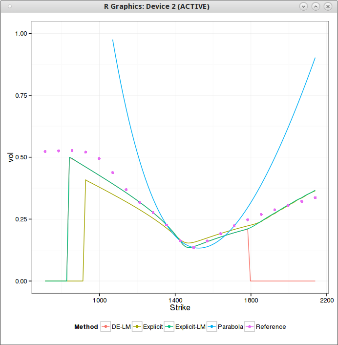
It's relatively well known that Heston does not fit the market for short expiries. Given that there are just 5 parameters to fit a full surface, it's almost logical that one part of the surface of it is not going to fit well the market. I was more surprised to see how bad Heston or Schobel-Zhu were to fit a single short expiry volatility slice. As an example I looked at SP500 options with 1 week expiry. It does not really matter if one forces kappa and rho to constant values (even to 0) the behavior is the same and the error in fit does not change much.
Schobel-Zhu fit for a slice of maturity 1 week
In this graph, the brown, green and red smiles corresponds to Schobel-Zhu fit using an explicit guess (matching skew & curvature ATM), using Levenberg-Marquardt on this guess, and using plain differential evolution. What happens is that the smiles flattens to quickly in the strike dimension. One consequence is that the implied volatility can not be computed for extreme strikes: the smile being too low, the price becomes extremely small, under machine epsilon and the numerical method (Cos) fails. There is also a bogus angle in the right wing, because of numerical error. I paid attention to ignore too small prices in the calibration by truncating the initial data.
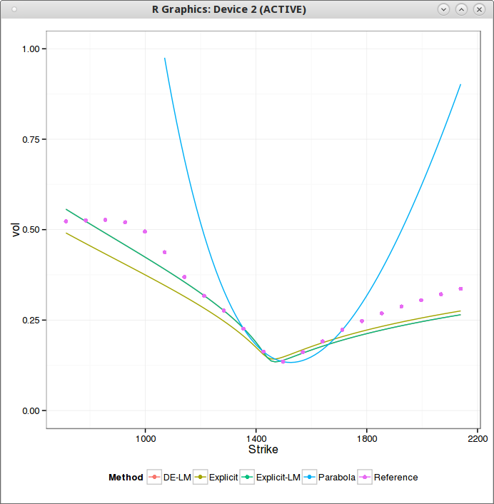
Heston fit, with Lord-Kahl (exact wings)
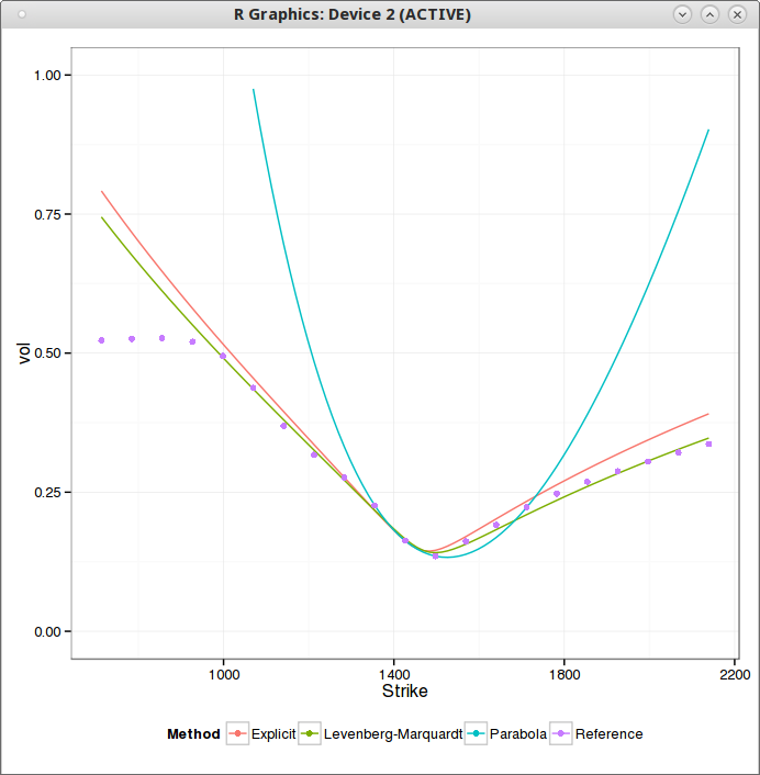
SABR behaves much better (fixing beta=1 in this case) in comparison (As I use the same truncation as for Schobel-Zhu, the flat left wing part is ignored).
SABR fit for a slice of maturity 1 week
For longer expiries, Heston & Schobel-Zhu, even limited to 3 parameters, actually give a better fit in general than SABR.
Most developers have strong opinions on dynamic types programming languages vs static types programming languages. The former is often assumed to be good for small projects/prototyping while the later better for bigger projects. But there is a surprisingly small number of studies to back those claims.
It's more interesting to look at generic types vs raw types use, where even less studies have been done. "Do developers benefit from generic types?: an empirical comparison of generic and raw types in java" concludes that generic types do not provide any advantages to fix typing errors, hardly surprising in my opinion. Generic types (especially with type erasure as in Java) is the typical idea that sounds good but that in practice does not really help: it makes the code actually more awkward to read and tend to make developers too lazy to create new classes that would often be more appropriate than a generic type (think Map<String,List<Map<String, Date>>>).
I have found a particularly nice initial guess to calibrate SABR. As it is quite close to the true best fit, it is tempting to use a very simple minimizer to go to the best fit. Levenberg-Marquardt works well on this problem, but can we shave off a few iterations?
I firstly considered the basic Newton's method, but for least squares minimization, the Hessian (second derivatives) is needed. It's possible to obtain it, even analytically with SABR, but it's quite annoying to derive it and code it without some automatic differentiation tool. It turns out that as I experimented with the numerical Hessian, I noticed that it actually did not help convergence in our problem. Gauss-Newton converges similarly (likely because the initial guess is good), and what's great about it is that you just need the Jacobian (first derivatives). Here is a good overview of Newton, Gauss-Newton and Levenberg-Marquardt methods.
While Gauss-Newton worked on many input data, I noticed it failed also on some long maturities equity smiles. The full Newton's method did not fare better. I had to take a close look at the matrices involved to understand what was going on. It turns out that sometimes, mostly when the SABR rho parameter is close to -1, the Jacobian would be nearly rank deficient (a row close to 0), but not exactly rank deficient. So everything would appear to work, but it actually misbehaves badly.
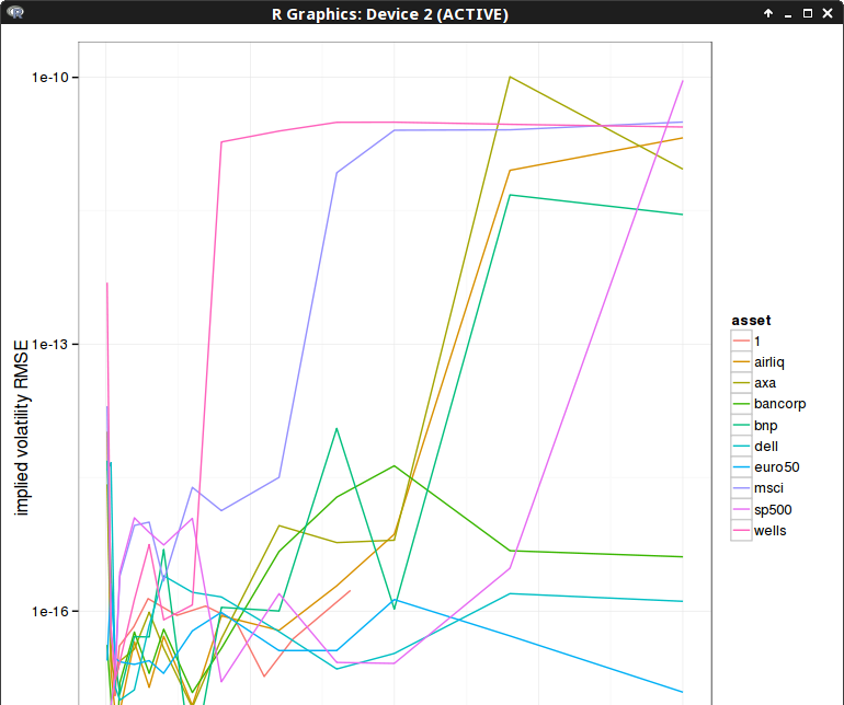
My first idea was to solve the reduced problem if a row of the Jacobian is too small, by just removing that row, and keep the previous value for the guess corresponding to that row. And this simplistic approach made the process work on all my input data. Here is the difference in RMSE compared to a highly accurate Levenberg-Marquardt minimization for 10 iterations:
Later, while reading some more material related to least square optimization, I noticed the use of the Moore-Penrose inverse in cases where a matrix is rank deficient. The Moore-Penrose inverse is defined as: $$ M^\star = V S^\star U^T$$ where \( S^\star \) is the diagonal matrix with inverted eigenvalues and 0 if those are deemed numerically close to 0, and \(U, V\) the eigenvectors of the SVD decomposition: $$M=U S V^T$$ It turns out to work very well, beside being simpler to code, I expected it to be more or less equivalent to the previous approach (a tiny bit slower but we don't care as we deal with small matrices, and the real slow part is the computation of the objective function and the Hessian, which is why looking at iterations is more important).
It seems to converge a little bit less quickly, likely due to the threshold criteria that I picked (1E-15). Three iterations is actually most of the time (90%) more than enough to achieve a good accuracy (the absolute RMSE is between 1E-4 and 5E-2) as the following graph shows. The few spikes near 1E-3 represent too large errors, the rest is accurate enough compared to the absolute RMSE.
To conclude, we have seen that using the Moore-Penrose inverse in a Gauss-Newton iteration allowed the Gauss-Newton method to work on rank-deficient systems. I am not sure how general that is, in my example, the true minimum either lies inside the region of interest, or on the border, where the system becomes deficient. Of course, this is related to a "physical" constraint, here namely rho > -1.