Arbitrage in Zeliade's SVI example
Zeliade wrote an excellent paper about the calibration of the SVI parameterization for the volatility surface in 2008. I just noticed recently that their example calibration actually contained strong calendar spread arbitrages. This is not too surprising if you look at the parameters, they vary wildly between the first and the second expiry.
| T | a | b | rho | m | s |
|---|---|---|---|---|---|
| 0.082 | 0.027 | 0.234 | 0.068 | 0.100 | 0.028 |
| 0.16 | 0.030 | 0.125 | -1.0 | 0.074 | 0.050 |
| 0.26 | 0.032 | 0.094 | -1.0 | 0.093 | 0.041 |
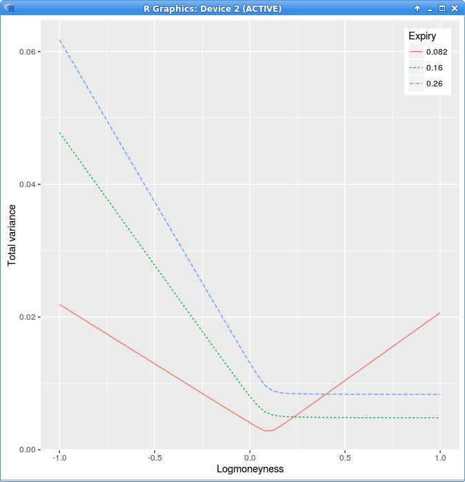
The calendar spread arbitrage is very visible in total variance versus log-moneyness graph:
in those coordinates if lines crosses, there is an arbitrage. This is because the total variance should be increasing with the expiry time.

Arbitrage in Zeliade's example
Why does this happen?
This is typically because the range of moneyness of actual market quotes for the first expiry is quite narrow, and looks more like a smile than a skew. The problem is that SVI is then quite bad at extrapolating this smile, likely because the SVI wings were used to fit well the curvature and have nothing to do with any actual market wings.
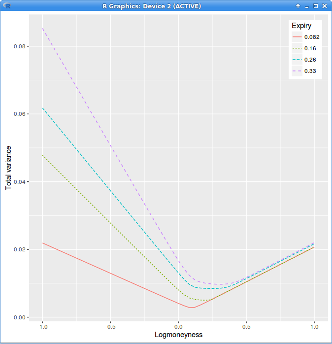
A consequence is that that the local volatility will be undefined in the right wing of the second and third expiries, if we keep the first expiry. It is interesting to look at what happens to the implied volatility if we decide either to:
- set the undefined local volatility to zero
- take the absolute value of the local variance
- search for the closest defined local volatility on the log-moneyness axis
- search for the closest positive local variance on the expiry axis and interpolate it linearly.

Total variance after flooring the local variance at zero.
Setting the undefined local volatility to zero makes the second, third, fourth expiry wings higher: the total variance is close to constant between expiries. One could have expected that a zero vol would lead to a lower implied vol, the opposite happens, because the original local vol is negative, so flooring it zero is like increasing it.
We can now deduce that taking the absolute value of the local variance is just going to push the implied variance even higher, and will therefore create a larger bias. Similarly, searching for closest local volatility is not going to improve anything.
Fixing the local volatility after the facts produces only a forward looking fix: the next expiries are going to be adjusted as a result.
Instead, in this example, the first maturity should be adjusted. A simple adjustment would be to cap the total variance of the first expiry so that it is never higher than the next expiry, before computing the local volatility. Although the resulting implied volatility will not be C2 or even C1 at the cap, the local volatility can be computed analytically on the left side, before the cap, and also analytically after the cap, on the right side. More care needs to be taken if the next expiry also needs to be capped (for example because there is another calendar spread arbitrage between expiry two and expiry three). In this case, the analytical calculation must be split in three zones: first-nocap + second-nocap, first-cap+second-nocap, first-cap+second-cap. So in reality having non C2 extrapolation can work well with local volatility if we are careful enough to avoid the artificial spike at the points of discontinuity.
There is yet another solution to produce a similar effect while still working at the local volatility level: if there is an arbitrage with the previous expiry at a given moneyness, we compute the local volatility ignoring the previous expiry (eventually extrapolating in constant manner) and we override the previous expiry local volatility for this moneyness. In terms of implied variance, this would correspond to removing the arbitrageable part of a given expiry, and replacing it with a linear interpolation between encompassing expiries, working backwards in time.