Shooting arbitrage - part I
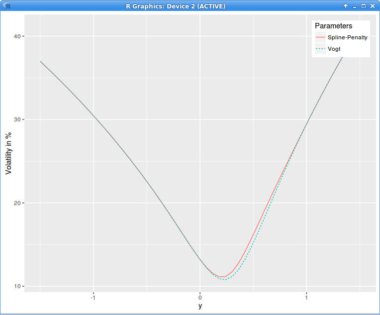
In my previous post, I looked at de-arbitraging volatilities of options of a specific maturity with SVI (re-)calibration. The penalty method can be used beyond SVI. For example I interpolate here with a cubic spline on 11 equidistant nodes the original volatility slice that contains arbitrages and then minimize with Levenberg-Marquardt and the negative local variance denominator penalty on 51 equidistant points. This results in a quite small adjustment to the original volatilities:

implied variance with Axel Vogt SVI parameters
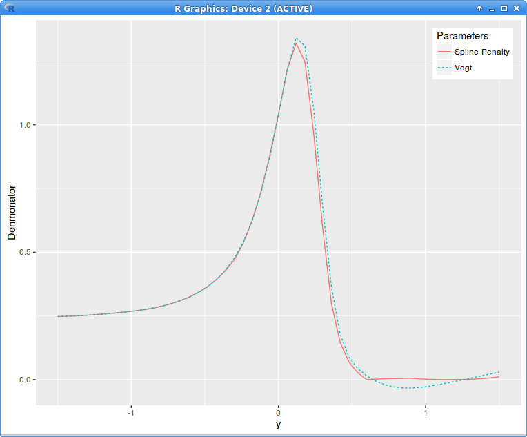
Interestingly the denominator looks almost constant, close to zero (in reality it is not constant, just close to zero, scales can be misleading):

local variance denominator g with Axel Vogt SVI parameters
The method does not work with too many nodes, for example 25 nodes was too much for the minimizer to do anything, maybe because there is too much interaction between nodes then.
I wondered then what would be the corresponding implied volatility for a constant denominator of 1E-4, glued to the implied volatility surface at the point where it reaches 1E-4. $$10^{-4}=1 - \frac{y}{w}\frac{\partial w}{\partial y} + \frac{1}{4}\left(-\frac{1}{4}-\frac{1}{w}+\frac{y^2}{w^2}\right)\left(\frac{\partial w}{\partial y}\right)^2 + \frac{1}{2}\frac{\partial^{2} w}{\partial y^2}$$
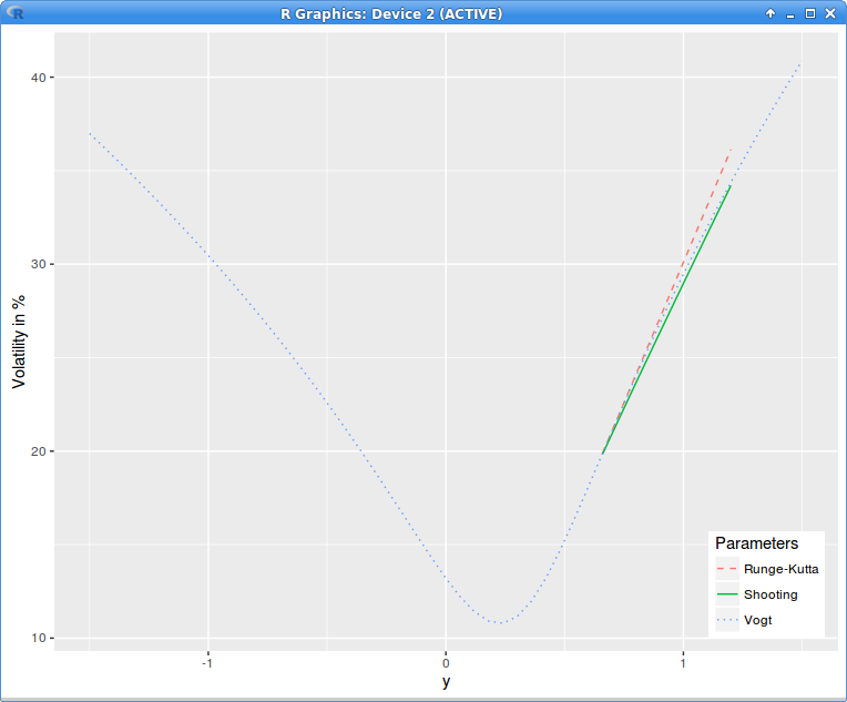
The equation can be easily solved with the Runge Kutta method by reducing it to a system of first order ordinary differential equations. As the following figure will show, as the initial conditions are the variance and the slope at the glueing point, the volatility is not continuous anymore at the next point where the denominator goes back to 1E-4. So this is only good if we replace the whole right wing: not so nice.
A simple idea is to adjust the initial slope so that the volatility is continuous at the next end-point. An ODE whose initial condition consists in the function values at two end-points is called a two-points boundary problem. A standard method to solve this kind of problem is just the basic simple idea and it is called the shooting method: we are shooting a projectile from point A so that it lands at point B. Any solver can be used so solve for the slope (secant, Newton, Brent, etc.).

implied variance with Axel Vogt SVI parameters
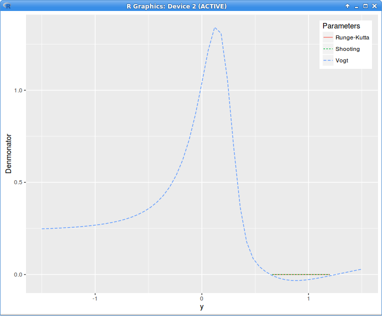
The volatility is only continuous, not C1 or C2 at A and B, but the local volatility is well defined and continuous, the denominator is just 1E-4 between A and B. The adjustments to the original volatilities is even smaller.
