Local Stochastic Volatility - Particles and Bins
In an earlier post, I mentioned the similarities between the Guyon-Labordere particle method and the Vanderstoep-Grzelak-Oosterlee “bin” method to calibrate and price under Local Stochastic volatility. I will be a bit more precise here. The same thing, really
The particle method can be seen as a generalization of the “bin” method. In deed, the bin method consists in doing the particle method using a histogram estimation of the conditional variance. The histogram estimation can be more or less seen as a very basic rectangle kernel with the appropriate bandwidth. The “bin” method is then just the particle method with another kernel (wiki link) (in the particle method, the kernel is a quartic with bandwidth defined by some slightly elaborate formula). A very good paper on this is Silverman Density estimation for statistics and data analysis, referenced by Guyon-Labordere.
In theory, the original particle method has the advantage of using a narrower bandwidth, resulting in a theoretical increase in performance as one does not have to sum over all particles, while providing a more local therefore precise estimate. In practice, the performance advantage is not so clear on my non optimized code. Two-pass There is an additional twist in the particle method: one can compute the expectation and the payoff evaluation in the same Monte-Carlo simulation, or in two sequential Monte-Carlo simulations.
Why would we do two? Mainly because the expectation is computed across all paths, at each time step, while, usually, payoff evaluation requires a full path as it will need to store some state at each observation time for path-dependent payoffs.
We can avoid recomputing the paths by just caching them at each observation time. The problem is that the size of this cache can quickly become extremely large and blow up the memory. For example a 10y daily knock-out will require 10 * 252 * 8 * 2 * MB = 40 GB for 1 million paths.
A side effect of the second simulation is that one can use a Quasi-Random number generator there, while for the first simulation, this is not easy as we compute all paths, dimension by dimension.
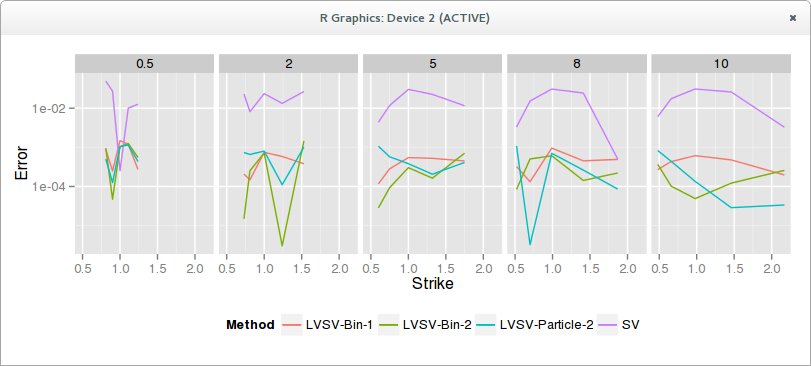
In practice, both methods work well, particle or bins, single-pass or two-pass. Here is a graph of the error in volatility, SV is a not so well calibrated Heston to market data. LVSV are the local stochastic volatility simulations, using as Vanderstoep 100 steps per year and 500K simulations with 30 bins.

The advantages of the particle do not show up in terms of accuracy on this example. I have also noticed that short expiries seem trickier, the error being larger. This might just be due to the time-step size, but interestingly the papers only show graphs of medium (min=6m) to large expiries.