Implying the Probability Density from Market Option Prices (Part 2)
This is a follow-up to my posts on the implied risk-neutral density (RND) of the SPW options before and after the big volatility change that happened in early February with two different techniques: a smoothing spline on the implied volatilities and a Gaussian kernel approach.
The Gaussian kernel (as well as to some extent the smoothing spline) let us believe that there are multiple modes in the distribution (multiple peaks in the density). In reality, Gaussian kernel approaches will, by construction, tend to exhibit such modes. It is not so obvious to know if those are real or artificial. There are other ways to apply the Gaussian kernel, for example by optimizing the nodes locations and the standard deviation of each Gaussian. The resulting density with those is very similar looking.
Following is the risk neutral density implied by nonic polynomial collocation out of the same quotes (Kees and I were looking at robust ways to apply the stochastic collocation):
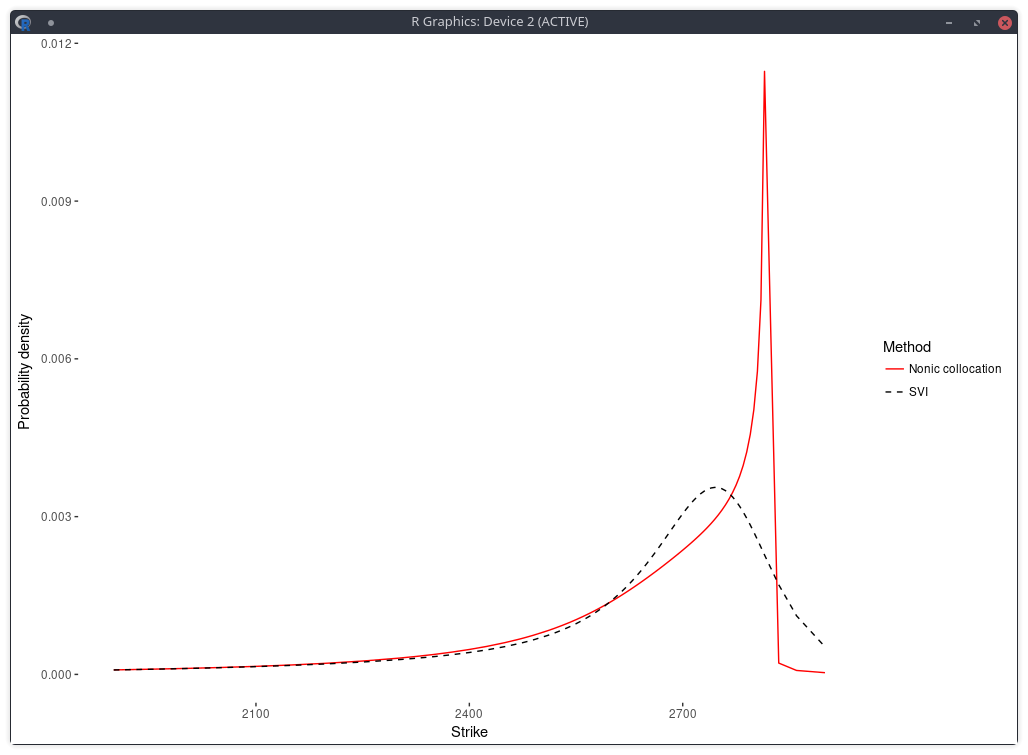
probability density of the SPX implied from 1-month SPW options with stochastic collocation on a nonic polynomial.
There is now just one mode, and the fit in implied volatilities is much better.
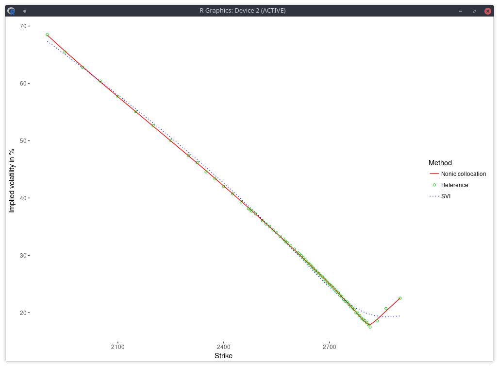
implied volatility of the SPX implied from 1-month SPW options with stochastic collocation on a nonic polynomial.
In a related experiment, Jherek Healy showed that the Andreasen-Huge arbitrage-free single-step interpolation will lead to a noisy RND. Sebastian Schlenkrich uses a simple regularization to calibrate his own piecewise-linear local volatility approximation (a Lamperti-transform based approximation instead of the single step PDE approach of Andreasen-Huge). His Tikhonov regularization consists here in applying a roughness penalty consisting in the sum of squares of the consecutive local volatility slope differences. This is nearly the same as using the matrix of discrete second derivatives as Tikhonov matrix. The same idea can be found in cubic spline smoothing. This roughness penalty can be added in the calibration of the Andreasen-Huge piecewise-linear discrete local volatilities and we obtain then a smooth RND:
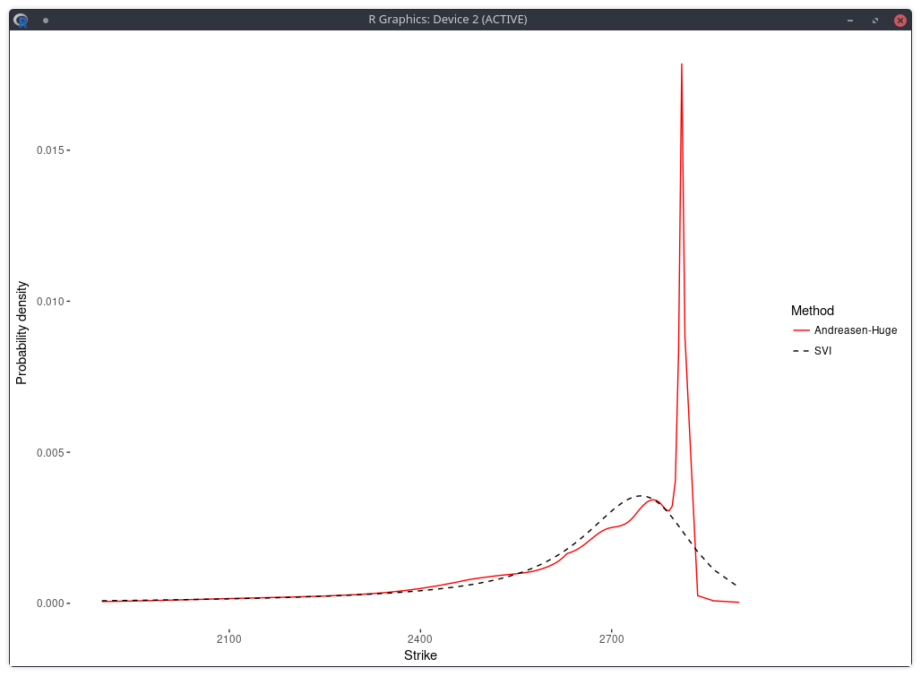
density of the SPX implied from 1-month SPW options with Andreasen-Huge and Tikhonov regularization.
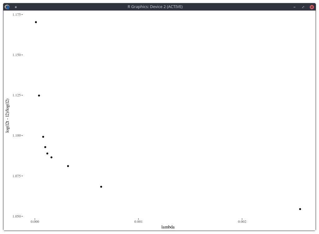
One difficulty however is to find the appropriate penalty factor \( \lambda \). On this example, the optimal penalty factor can be guessed from the L-curve which consists in plotting the L2 norm of the objective against the L2 norm of the penalty term (without the factor lambda) in log-log scale, see for example this document. Below I plot a closely related function: the log of the penalty (with the lambda factor) divided by the log of the objective, against lambda. The point of highest curvature corresponds to the optimal penalty factor.
density of the SPX implied from 1-month SPW options with nodes located at every 2 market strike.
Note that in practice, this requires multiple calibrations the model with different values of the penalty factor, which can be slow. Furthermore, from a risk perspective, it will also be challenging to deal with changes in the penalty factor.
The error of model versus market implied volatilies is similar to the nonic collocation (not better) even though the shape is less smooth and, a priori, less constrained as, on this example, the Andreasen-Huge method has 75 free-parameters while the nonic collocation has 9.