Flat Volatility Surfaces & Discrete Dividends
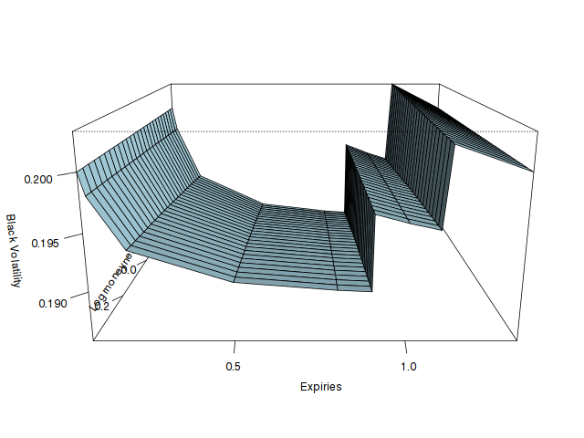
In papers around volatility and cash (discrete) dividends, we often encounter the example of the flat volatility surface. For example, the OpenGamma paper presents this graph:It shows that if the Black volatility surface is fully flat, there are jumps in the pure volatility surface (corresponding to a process that includes discrete dividends in a consistent manner) at the dividend dates or equivalently if the pure volatility surface is flat, the Black volatility jumps.
This can be traced to the fact that the Black formula does not respect C(S,K,Td-) = C(S,K-d,Td) as the forward drops from F(Td-) to F(Td-)-d where d is dividend amount at td, the dividend ex date.
Unfortunately, those examples are not very helpful. In practice, the market observables are just Black volatility points, which can be interpolated to volatility slices for each expiry without regards to dividends, not a full volatility surface. Discrete dividends will mostly happen between two slices: the Black volatility jump will happen on some time-interpolated data.
While the jump size is known (it must obey to the call price continuity), the question of how one should interpolate that data until the jump is far from trivial even using two flat Black volatility slices.
The most logical is to consider a model that includes discrete dividends consistently. For example, one can fully lookup the Black volatility corresponding the price of an option assuming a piecewise lognormal process with jumps at the dividend dates. It can be priced by applying a finite difference method on the PDE. Alternatively, Bos & Vandermark propose a simple spot and strike adjusted Black formula that obey the continuity requirement (the Lehman model), which, in practice, stays quite close to the piecewise lognormal model price. Another possibility is to rely on a forward modelling of the dividends, as in Buehler (if one is comfortable with the idea that the option price will then depend ultimately on dividends past the option expiry).
Recently, a Wilmott article suggested to only rely on the jump adjustment, but did not really mention how to find the volatility just before or just after the dividend. Here is an illustration of how those assumptions can change the volatility in between slices using two dividends at T=0.9 and T=1.1.
In the first graph, we just interpolate linearly in forward moneyness the pure vol from the Bos & Vandermark formula, as it should be continuous with the forward (the PDE would give nearly the same result) and compute the equivalent Black volatility (and thus the jump at the dividend dates).
In the second graph, we interpolate linearly the two Black slices, until we find a dividend, at which point we impose the jump condition and repeat the process until the next slice. We process forward (while the Wilmott article processes backward) as it seemed a bit more natural to make the interpolation not depend on future dividends. Processing backward would just make the last part flat and first part down-slopping. On this example backward would be closer to the Bos Black volatility, but when the dividends are near the first slice, the opposite becomes true.
While the scale of those changes is not that large on the example considered, the choice can make quite a difference in the price of structures that depend on the volatility in between slices. A recent example I encountered is the variance swap when one includes adjustment for discrete dividends (then the prices just after the dividend date are used).
To conclude, if one wants to use the classic Black formula everywhere, the volatility must jump at the dividend dates. Interpolation in time is then not straightforward and one will need to rely on a consistent model to interpolate. It is not exactly clear then why would anyone stay with the Black formula except familiarity.


