Clenshaw-Curtis Quadrature Implementation by FFT in Practice

Wed, Sep 27, 2023

The Clenshaw-Curtis quadrature is known to be competitive with Gauss quadratures. It has several advantages:

• the weights are easy and fast to compute.
• adaptive / doubling quadratures are possible with when the Chebyshev polynomial of the second kind is used for the quadrature.
• the Chebyshev nodes may also be used to interpolate some costly function.

The wikipedia article has a relatively detailed description on how to compute the quadrature weights corresponding to the Chebyshev polynomial of the second kind (where the points -1 and 1 are included), via a type-I DCT. It does not describe the weights corresponding to the Chebyshev polynomials of the first kind (where -1 and 1 are excluded, like the Gauss quadratures). The numbersandshapes blog post describes it very nicely. There are some publications around computation of Clenshaw-Curtis or Fejer rules, a recent one is Fast construction of Fejér and Clenshaw–Curtis rules for general weight functions.

I was looking for a simple implementation of the quadrature or its weights, leveraging some popular FFT library such as fftw (The Fastest Fourier Transform in the West). I expected it to be a simple search. Instead, it was surprisingly difficult to find even though the code in Julia consists only in a few lines:

• First kind (following the numbersandshapes blog post)

  chebnodes(T, n::Int) = @. (cos(((2:2:2n) - 1) * T(pi) / 2n))
  x = chebnodes(Float64, N)
  m = vcat(sqrt(2), 0.0, [(1 + (-1)^k) / (1 - k^2) for k = 2:N-1])
  ws = sqrt(2 / N) * idct(m)

• Second kind (the classic Clenshaw-Curtis, following some article from Treffenden)

  cheb2nodes(T, n::Int) = @. (cos(((0:n-1)) * T(pi) / (n-1)))
  x = cheb2nodes(Float64, N)
  c = vcat(2, [2 / (1 - i^2) for i = 2:2:(N-1)]) # Standard Chebyshev moments
  c = vcat(c, c[Int(floor(N / 2)):-1:2])         # Mirror for DCT via FFT 
  ws = real(ifft(c))                             # Interior weight
  ws[1] /= 2
  ws = vcat(ws, ws[1])                           # Boundary weights

There are some obvious possible improvements: the nodes are symmetric and only need to be computed up to N/2, but the above is quite fast already. The Julia package FastTransforms.jl provides the quadrature weights although the API is not all that intuitive:

• First kind:

   fejer1weights(FastTransforms.chebyshevmoments1(Float64,N))

• Second kind:

   clenshawcurtisweights(FastTransforms.chebyshevmoments1(Float64,N))

Interestingly the first kind is twice faster with FastTransforms, which suggests a similar symetry use as for the second kind. But the second kind is nearly twice slower.

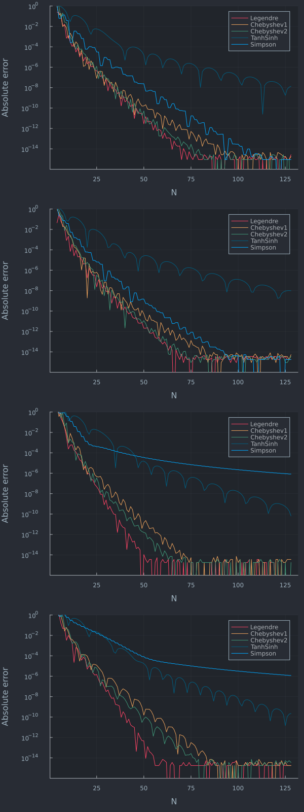
Although Clenshaw-Curtis quadratures are appealing, the Gauss-Legendre quadrature is often slightly more accurate on many practical use cases and there exists also fast enough ways to compute its weights. For example, in the context of a two-asset basket option price using a vol of 20%, strike=spot=100, maturity 1 year, and various correlations we have the below error plots