Brownian Bridge and Discrete Random Variables
The new Heston discretisation scheme I wrote about a few weeks ago makes use a discrete random variable matching the first five moments of the normal distribution instead of the usual normally distributed random variable, computed via the inverse cumulative distribution function. Their discrete random variable is: $$\xi = \sqrt{1-\frac{\sqrt{6}}{3}} \quad \text{ if } U_1 < 3,,$$ $$ \xi =-\sqrt{1-\frac{\sqrt{6}}{3}} \quad \text{ if } U_1 > 4,,$$ $$\xi = \sqrt{1+\sqrt{6}} \quad \text{ if } U_1 = 3,,$$ $$\xi = -\sqrt{1+\sqrt{6}} \quad \text{ if } U_1 = 4,,$$ with \(U_1 \in \{0,1,…,7\}\)
The advantage of the discrete variable is that it is much faster to generate. But there are some interesting side-effects. The first clue I found is a loss of accuracy on forward-start vanilla options.
By accident, I found a much more interesting side-effect: you can not use the Brownian-Bridge variance reduction on the discrete random variable. This is very well illustrated by the case of a digital option in the Black model, for example with volatility 10% and a 3 months maturity, zero interest rate and dividends. For the following graph, I use 16000 Sobol paths composed of 100 time-steps.
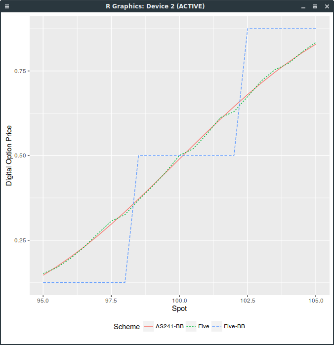
Digital Call price with different random variables.
The “-BB” suffix stands for the Brownian-Bridge path construction, “Five” for five moments discrete variable and “AS241” for the inverse cumulative distribution function (continuous approach). As you can see, the price is discrete, and follows directly from the discrete distribution. The use of any random number generator with a large enough number of paths would lead to the same conclusion.
This is because with the Brownian-Bridge technique, the last point in the path, corresponding to the maturity, is sampled first, and the other path points are then completed inside from the first and last points. But the digital option depends only on the value of the path at maturity, that is, on this last point. As this point corresponds follows our discrete distribution, the price of the digital option is a step function.
In contrast, for the incremental path construction, each point is computed from the previous point. The last point will thus include the variation of all points in the path, which will be very close to normal, even with a discrete distribution per point.
The take-out to price more exotic derivatives (including forward-start options) with discrete random variables and the incremental path construction, is that several intermediate time-steps (between payoff observations) are a must-have with discrete random variables, however small is the original time-step size.
Furthermore, one can notice the discrete staircase even with a relavely small time-step for example of 1/32 (meaning 8 intermediate time-steps in our digital option example). I suppose this is a direct consequence of the digital payoff discontinuity. In Talay “Efficient numerical schemes for the approximation of expectations of functionals of the solution of a SDE, and applications” (which you can read by adding .sci-hub.cc to the URL host name), second order convergence is proven only if the payoff function and its derivatives up to order 6 are continuous. There is something natural that a discrete random variable imposes continuity conditions on the payoff, not necessary with a continuous, smooth random variable: either the payoff or the distribution needs to be smooth.