Almost Explicit Implied Volatility
Several years ago, I had explored accuracy and performance of different ways to imply the Black-Scholes volatility. Jherek Healy proposed some improvements over my naive algorithm on his blog. Recently, a Linkedin post mentioned a new paper from Wolfgang Schadner which presents an almost explicit formula for the implied volatility. Almost because it actually relies on some implementation of the quantile function for the inverse Gaussian distribution: it requires a specialized numerical algorithm in practice, such as the one from Giner and Smyth.
The idea is actually not new, the same formula has been used back in 2016 by Jaehyuk Choi in his github repository. If we have a good inverse Gaussian distribution function, the algorithm is clean and simple:
using Distributions
export impliedVolatilityIG
const N = Normal()
function impliedVolatilityIG(isCall::Bool, price::T, forward, strike,  timeToExpiry, df) where {T}
    c, ex = normalizePrice(isCall, price, forward, strike, df)
    if c >= 1 / ex || c >= 1
        throw(DomainError(c, string("price higher than intrinsic value ", 1 / ex)))
    elseif c <= 0
        throw(DomainError(c, "price is negative"))
    end
    x = log(ex)
    return if abs(x) < 4 * eps(T)
        2 * quantile(N, (c + 1) / 2) / sqrt(timeToExpiry)
    else
        mu = 2 / abs(x)
        u = cquantile(InverseGaussian(mu), c)
        2 / sqrt(u * timeToExpiry)
    end
end
reusing the price normalization idea of Li.
function normalizePrice(isCall::Bool, price, f, strike, df)
    c = price / (f * df)
    ex = f / strike
    if !isCall
        if ex <= 1
            c = c + 1 - 1 / ex # put call parity
        else #duality + put call parity
            c = ex * c
            ex = 1 / ex
        end
    else
        if ex > 1 # use c(-x0, v)
            c = (f * (c - 1) + strike) / strike # in out duality, c = ex*c + 1 - ex
            ex = 1 / ex
        end
    end
    return c, ex
end
I was wondering how accurate it was especially for very out-of-the-money options, and how fast it was in practice. Below I compare various implementations in Julia:
- Peter Jaeckel, which is arguably the industry standard.
- Jherek Healy, which consists in (log-)Householder iterations on top of a good explcit initial guess.
- The inverse Gaussian approach using Julia’s Distribution.jl package (as in the above code).
- The inverse Gaussian approach using a basic port of statsmod R algorithm, adapted to compute the complementary quantile function. This corresponds to a different implementation of
cquantile(InverseGaussian(mu),c).
I consider call optiun prices for a fixed strike K = 200 for a forward F = 100, and a time to maturity T = 1.0 year, varying the volatility from 0.02 to 4.0 in steps of 0.01. This constitute 399 samples.
| Algorithm | vol RMSD | vol MAXAD | Price MAXAD | Rel. Price MAXAD | Time |
|---|---|---|---|---|---|
| Jaeckel | 8.66e-16 | 4.00e-15 | 4.26e-14 | 1.81e-12 | 104 μs |
| Healy | 1.57e-15 | 9.77e-15 | 8.53e-14 | 3.02e-10 | 107 μs |
| IG Distribution | 7.37e-16 | 5.41e-15 | 2.84e-14 | 8.99e-11 | 246 μs |
| IG statsmod | 7.77e-16 | 7.55e-15 | 8.24e-13 | 3.03e-10 | 311 μs |
The inverse Gaussian approach is competitive but still twice slower than Peter Jaeckel’s algorithm on this example. How does the error in volatility actually look like?
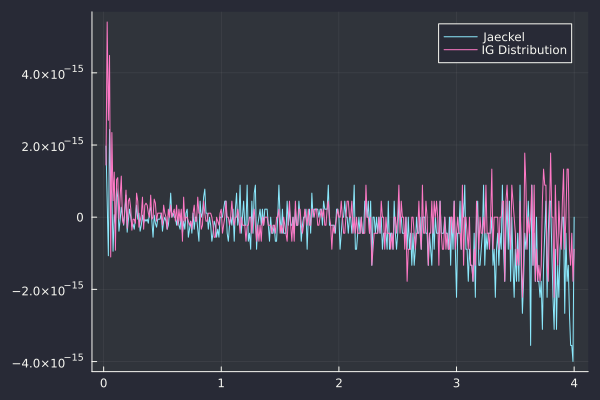
Error in impled volatility of the various algorithms
The accuracy of the inverse Gaussian looks as good as Jackel’s algorithm, when using Julia’s package Distibutions.jl (it is slightly less accurate towards low vol, but slightly more accurate for high vols).
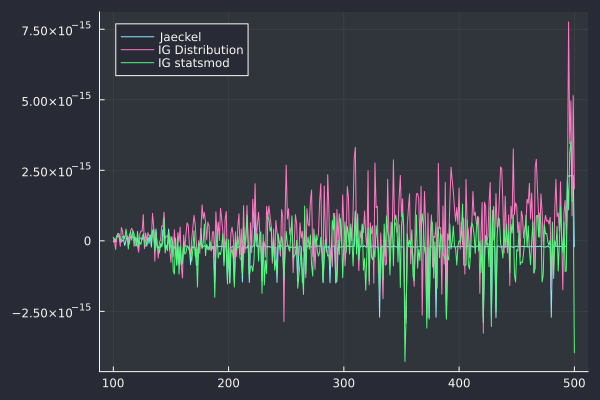
It is revealing to also look at the case of varying strikes for a fixed volatility. We consider a volatility fixed to 0.1 (or 10%) and vary the strike from 100 to 500 by steps of 1.
| Algorithm | vol RMSD | vol MAXAD | Price MAXAD | Rel. Price MAXAD | Time |
|---|---|---|---|---|---|
| JAECKEL | 6.50e-16 | 2.73e-15 | 7.11e-15 | 6.59e-12 | 154 μs |
| HEALY | 6.56e-16 | 2.73e-15 | 3.55e-14 | 6.59e-12 | 110 μs |
| IG Distribution | 1.21e-15 | 7.76e-15 | 1.78e-14 | 1.95e-11 | 1704 μs |
| IG statsmod | 8.68e-16 | 4.27e-15 | 1.06e-14 | 1.32e-11 | 288 μs |
On this example the Julia Distributions.jl leads to a performance degradation by a factor of 10 and is less accurate. It would be worth investigating exactly where lies the bottleneck, as statsmod custom implementation keeps a good performance profile.