Adjoint algorithmic differentiation is particularly interesting in finance as we often encounter the case of a function that takes many input (the market data) and returns one output (the price) and we would like to also compute sensitivities (greeks) to each input.
As I am just starting around it, to get a better grasp, I first tried to apply the idea to the analytic knock out barrier option formula, by hand, only to find out I was making way too many errors by hand to verify anything. So I tried the simpler vanilla Black-Scholes formula. I also made various errors, but managed to fix all of them relatively easily.
I decided to compare how much time it took to compute price, delta, vega, theta, rho, rho2 between single sided finite difference and the adjoint approach. Here are the results for 1 million options:
FD time=2.13s Adjoint time=0.63s
It works well, but doing it by hand is crazy and too error prone. It might be simpler for Monte-Carlo payoffs however.
There are not many Java tools that can do reverse automatic differentiation, I found some thesis on it, with an interesting byte code oriented approach (one difficulty is that you need to reverse loops, while statements).
At the same time, Tavella and Randall show in their book that numerically, placing the strike in the middle of two nodes leads to a more accurate result. My own numerical experiments confirm Tavella and Randall suggestion.
In reality, what Pooley et al. really mean, is that quadratic convergence is maintained if the strike is on the grid for vanilla payoffs, contrary to the case of discontinuous payoffs (like digital options) where the convergence decreases to order 1. So it's ok to place the strike on the grid for a vanilla payoff, but it's not optimal, it's still better to place it in the middle of two nodes. Here are absolute errors in a put option price:
on grid, no smoothing 0.04473021824995271 on grid, Simpson smoothing 0.003942854282069419 on grid, projection smoothing 0.044730218065351934 middle, no smoothing 0.004040359609906119
As expected (and mentioned in Pooley et al.), the projection does not do anything here. When the grid size is doubled, the convergence ratio of all methods is the same (order 2), but placing the strike in the middle still increases accuracy significantly.
Here is are the same results, but for a digital put option: on grid, no smoothing 0.03781319921461046 on grid, Simpson smoothing 8.289052335705427E-4 on grid, projection smoothing 1.9698293587372406E-4 middle, no smoothing 3.5122153011418744E-4
Here only the 3 last methods are of order-2 convergence, and projection is in deed the most accurate method, but placing the strike in the middle is really not that much worse, and much simpler.
Recently, I noticed how close are the two PDE based approaches from Andreasen-Huge and Hagan for an arbitrage free SABR. Hagan gives a local volatility very close to the one Andreasen-Huge use in the forward PDE in call prices. A multistep Andreasen-Huge (instead of their one step PDE method) gives back prices and densities nearly equal to Hagan density based approach.
Hagan proposed in some unpublished paper a coordinate transformation for two reasons: the ideal range of strikes for the PDE can be very large, and concentrating the points where it matters should improve stability and accuracy. The transform itself can be found in the Andersen-Piterbarg book “Interest Rate Modeling”, and is similar to the famous log transform, but for a general local volatility function (phi in the book notation).
There are two ways to transform Andreasen Huge PDE:
through a non-uniform grid: the input strikes are directly transformed based on a uniform grid in the inverse transformed grid (paying attention to still put the strike in the middle of two points). This is detailed in the Andersen-Piterbarg book.
through a variable transform in the PDE: this gives a slightly different PDE to solve. One still needs to convert then a given strike, to the new PDE variable. This kind of transform is detailed in the Tavella-Randall book “Pricing Financial Instruments: the Finite Difference Method”, for example.
Both are more or less equivalent. I would expect the later to be slightly more precise but I tried the former as it is simpler to test if you have non uniform parabolic PDE solvers.
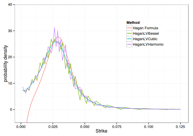
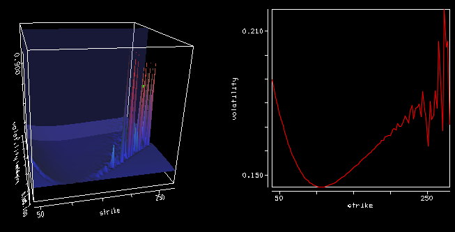
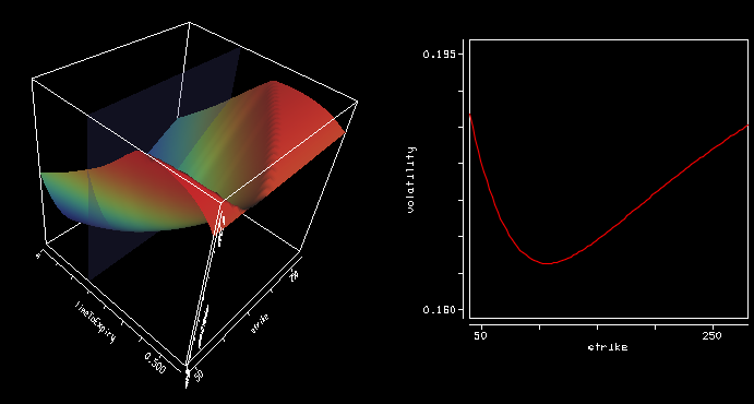
It works very well, but I found an interesting issue when computing the density (second derivative of the call price): if one relies on a Hermite kind of spline (Bessel/Parabolic or Harmonic), the density wiggles around. The C2 cubic spline solves this problem as it is C2. Initially I thought those wiggles could be produced because the interpolation did not respect monotonicity and I tried a Hyman monotonic cubic spline out of curiosity, it did not change anything (in an earlier version of this post I had a bug in my Hyman filter) as it preserves monotonicity but not convexity. The wiggles are only an effect of the approximation of the derivatives value.
Initially, I did not notice this on the uniform discretization mostly because I used a large number of strikes in the PDE (here I use only 50 strikes) but also because the effect is somewhat less pronounced in this case.
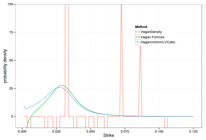
I also discovered a bug in my non uniform implementation of Hagan Density PDE, I forgot to take into account an additional dF/dz factor when the density is integrated. As a result, the density was garbage when computed by a numerical difference.
HaganDensity denotes the transformed PDE on density approach. Notice the non-sensical spikes
Bad Call prices around the forward with Hagan Density PDE. Notice the jumps.
Today, after wondering why my desktop computer became so unstable (frequent crashes under Fedora), I found out that the micro usb port of my cell phone has some kind of short circuit. My phone behaves strangely in 2014, it lasted nearly 1 week on battery (I lost it for half of the week), and seems to shutdown for no particular reason once in a while.
On the positive side, I also discovered, after owning my monitor for around 5 years, that it has SD card slots on the side, as well as USB ports. I always used the USB ports of my desktop and never really looked at the side of my monitor…
I also managed to seriously boost the speed of my home network with a cheap TP-Link wifi router. The one included in the ISP box-modem only supported 802.11g and had really crap coverage, so crap that it was seriously limiting the internet traffic. In the end it was just a matter of disabling wifi and DHCP on the box, adding the new router in the DMZ, and adding a static WAN IP for the box in the router configuration. I did not realize how much of a difference this could make, even on simple websites. I was also surprised that, for some strange reason, routers are cheaper than access points these days.
The Fortran minpack library has a good Levenberg-Marquardt minimizer, so good, that it has been ported to many programming languages. Unfortunately it does not support contraints, even simple bounds.
One way to achieve this is to transform the domain via a bijective function. For example, \(a+\frac{b-a}{1+e^{-\alpha t}}\) will transform \(]-\infty, +\infty[\) to ]a,b[. Then how should one choose \(\alpha\)?
A large \(\alpha\) will make tiny changes in \(t\) appear large. A simple rule is to ensure that \(t\) does not create large changes in the original range ]a,b[, for example we can make \(\alpha t \leq 1\), that is \( \alpha t= \frac{t-a}{b-a} \).
In practice, for example in the calibration of the Double-Heston model on real data, a naive \( \alpha=1 \) will converge to a RMSE of 0.79%, while our choice will converge to a RMSE of 0.50%. Both will however converge to the same solution if the initial guess is close enough to the real solution. Without any transform, the RMSE is also 0.50%. The difference in error might not seem large but this results in vastly different calibrated parameters. Introducing the transform can significantly change the calibration result, if not done carefully.
Another simpler way would be to just impose a cap/floor on the inputs, thus ensuring that nothing is evaluated where it does not make sense. In practice, it however will not always converge as well as the unconstrained problem: the gradient is not defined at the boundary. On the same data, the Schobel-Zhu, unconstrained converges with RMSE 1.08% while the transform converges to 1.22% and the cap/floor to 1.26%. The Schobel-Zhu example is more surprising since the initial guess, as well as the results are not so far:
Initial volatility (v0)
18.1961174789
Long run volatility (theta)
1
Speed of mean reversion (kappa)
101.2291161766
Vol of vol (sigma)
35.2221829015
Correlation (rho)
-73.7995231799
ERROR MEASURE
1.0614889526
Initial volatility (v0)
17.1295934569
Long run volatility (theta)
1
Speed of mean reversion (kappa)
67.9818356373
Vol of vol (sigma)
30.8491256097
Correlation (rho)
-74.614636128
ERROR MEASURE
1.2256421987
The initial guess is kappa=61% theta=11% sigma=26% v0=18% rho=-70%. Only the kappa is different in the two results, and the range on the kappa is (0,2000) (it is expressed in %), much larger than the result. In reality, theta is the issue (in (0,1000)). Forbidding a negative theta has an impact on how kappa is picked. The only way to be closer
Finally, a third way is to rely on a simple penalty: returning an arbitrary large number away from the boundary. In our examples this was no better than the transform or the cap/floor.
Trying out the various ways, it seemed that allowing meaningless parameters, as long as they work mathematically produced the best results with Levenberg-Marquardt, particularly, allowing for a negative theta in Schobel-Zhu made a difference.
One way is due to Andreasen and Huge, where they find an equivalent local volatility expansion, and then use a one-step finite difference technique to price.
The other way is due to Hagan himself, where he numerically solves an approximate PDE in the probability density, and then price with options by integrating on this density.
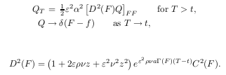
It turns out that the two ways are much closer than I first thought. Hagan PDE in the probability density is actually just the Fokker-Planck (forward) equation.
The \(\alpha D(F)\) is just the equivalent local volatility. Andreasen and Huge use nearly the same local volatility formula but without the exponential part (that is often negligible except for long maturities), directly in Dupire forward PDE:
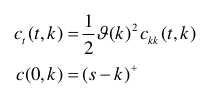
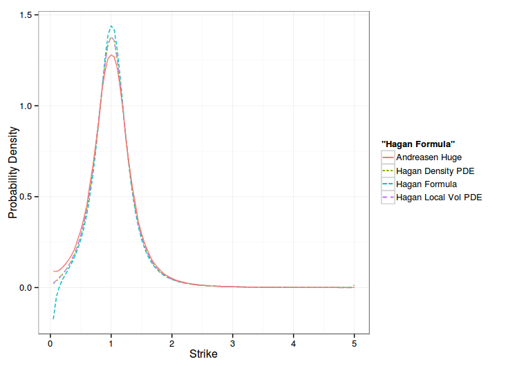
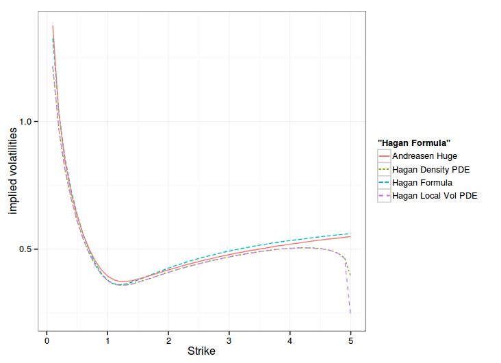
A common derivation (for example in Gatheral book of the Dupire forward PDE is to actually use the Fokker-Planck equation in the probability density integral formula. Out of curiosity, I tried to price direcly with Dupire forward PDE and the Hagan local volatility formula, using just linear boundary conditions. Here are the results on Hagan own example:
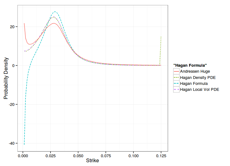
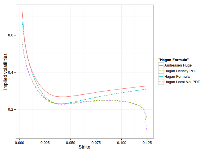
The Local Vol direct approach overlaps the Density approach nearly exactly, except at the high strike boundary, when it comes to probability density measure or to implied volatility smile. On Andreasen and Huge data, it gives the following:
One can see that the one step method approximation gives the overall same shape of smile, but shifted, while the PDE, in local vol or density matches the Hagan formula at the money.
Hagan managed to derive a slightly more precise local volatility by going through the probability density route, and his paper formalizes his model in a clearer way: the probability density accumulates at the boundaries. But in practice, this formalism does not seem to matter. The forward Dupire way is more direct and slightly faster. This later way also allows to use alternative boundaries, like Andreasen-Huge did.
Prices of a Future contract and a Forward contract are the same under the Black-Scholes assumptions (deterministic rates) but the price of options on Futures or options on Forwards might still differ. I did not find this obvious at first.
For example, when the underlying contract expiration date (Futures, Forward) is different from the option expiration date. For a Future Option, the Black-76 formula can be used, the discounting is done from the option expiry date, because one receives the cash on expiration due to the margin account. For a Forward Option, the discounting need to be done from the Forward contract expiry date.
European options prices will be the same when the underlying contract expiration date is the same as the option expiration date. However, this is not true for American options: the immediate exercise will need to be discounted to the Forward expiration date for a Forward underlying, not for a Future.
Using precise vanilla option pricing engine for Heston or Schobel-Zhu, like the Cos method with enough points and a large enough truncation can still lead to spikes in the Dupire local volatility (using the variance based formula).
Local volatility
Implied volatility
The large spikes in the local volatility 3d surface are due to constant extrapolation, but there are spikes even way before the extrapolation takes place at longer maturities. Even if the Cos method is precise, it seems to be not enough, especially for large strikes so that the second derivative over the strike combined with the first derivative over time can strongly oscillate.
After wondering about possible solutions (using a spline on the implied volatilities), the root of the error was much simpler: I used a too small difference to compute the numerical derivatives (1E-6). Moving to 1E-4 was enough to restore a smooth local volatility surface.
I always imagined local stochastic volatility to be complicated, and thought it would be very slow to calibrate.
After reading a bit about it, I noticed that the calibration phase could just consist in calibrating independently a Dupire local volatility model and a stochastic volatility model the usual way.
One can then choose to compute on the fly the local volatility component (not equal the Dupire one, but including the stochastic adjustment) in the Monte-Carlo simulation to price a product.
There are two relatively simple algorithms that are remarkably similar, one by Guyon and Henry-Labordère in "The Smile Calibration Problem Solved":
In the particle method, the delta function is a regularizing kernel approximating the Dirac function. If we use the notation of the second paper, we have a = psi.
The methods are extremely similar, the evaluation of the expectation is slightly different, but even that is not very different. The disadvantage is that all paths are needed at each time step. As a payoff is evaluated over one full path, this is quite memory intensive.
I did some experiments fitting Heston, Schobel-Zhu, Bates and Double-Heston to a real world equity index implied volatility surface. I used a global optimizer (differential evolution).
To my surprise, the Heston fit is quite good: the implied volatility error is less than 0.42% on average. Schobel-Zhu fit is also good (0.47% RMSE), but a bit worse than Heston. Bates improves quite a bit on Heston although it has 3 more parameters, we can see the fit is better for short maturities (0.33% RMSE). Double-Heston has the best fit overall but it is not that much better than simple Heston while it has twice the number of parameters, that is 10 (0.24 RMSE). Going beyond, for example Triple-Heston, does not improve anything, and the optimization becomes very challenging. With Double-Heston, I already noticed that kappa is very low (and theta high) for one of the processes, and kappa is very high (and theta low) for the other process: so much that I had to add a penalty to enforce constraints in my local optimizer. The best fit is at the boundary for kappa and theta. So double Heston already feels over-parameterized.
Heston volatility error
Schobel-Zhu volatility error
Bates volatility error
Double Heston volatility error
Another advantage of Heston is that one can find tricks to find a good initial guess for a local optimizer.
Update October 7: My initial fit relied only on differential evolution and was not the most stable as a result. Adding Levenberg-Marquardt at the end stabilizes the fit, and improves the fit a lot, especially for Bates and Double Heston. I updated the graphs and conclusions accordingly. Bates fit is not so bad at all.