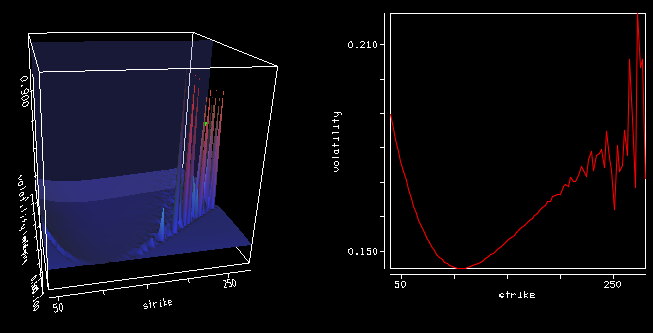
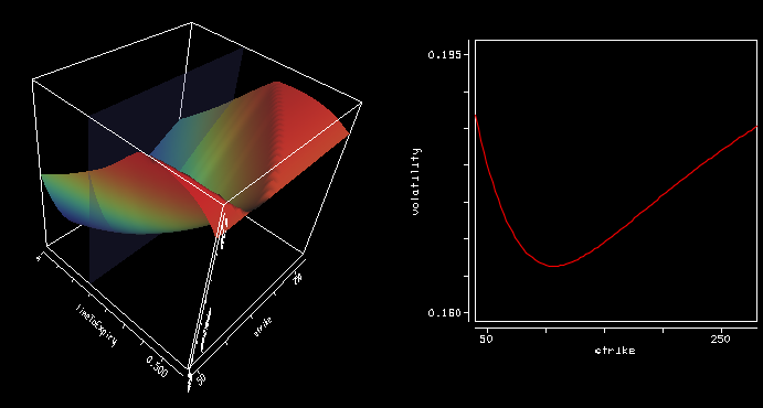
Using precise vanilla option pricing engine for Heston or Schobel-Zhu, like the Cos method with enough points and a large enough truncation can still lead to spikes in the Dupire local volatility (using the variance based formula).
Local volatility
Implied volatility
The large spikes in the local volatility 3d surface are due to constant extrapolation, but there are spikes even way before the extrapolation takes place at longer maturities. Even if the Cos method is precise, it seems to be not enough, especially for large strikes so that the second derivative over the strike combined with the first derivative over time can strongly oscillate.
After wondering about possible solutions (using a spline on the implied volatilities), the root of the error was much simpler: I used a too small difference to compute the numerical derivatives (1E-6). Moving to 1E-4 was enough to restore a smooth local volatility surface.
I always imagined local stochastic volatility to be complicated, and thought it would be very slow to calibrate.
After reading a bit about it, I noticed that the calibration phase could just consist in calibrating independently a Dupire local volatility model and a stochastic volatility model the usual way.
One can then choose to compute on the fly the local volatility component (not equal the Dupire one, but including the stochastic adjustment) in the Monte-Carlo simulation to price a product.
There are two relatively simple algorithms that are remarkably similar, one by Guyon and Henry-Labordère in "The Smile Calibration Problem Solved":
In the particle method, the delta function is a regularizing kernel approximating the Dirac function. If we use the notation of the second paper, we have a = psi.
The methods are extremely similar, the evaluation of the expectation is slightly different, but even that is not very different. The disadvantage is that all paths are needed at each time step. As a payoff is evaluated over one full path, this is quite memory intensive.
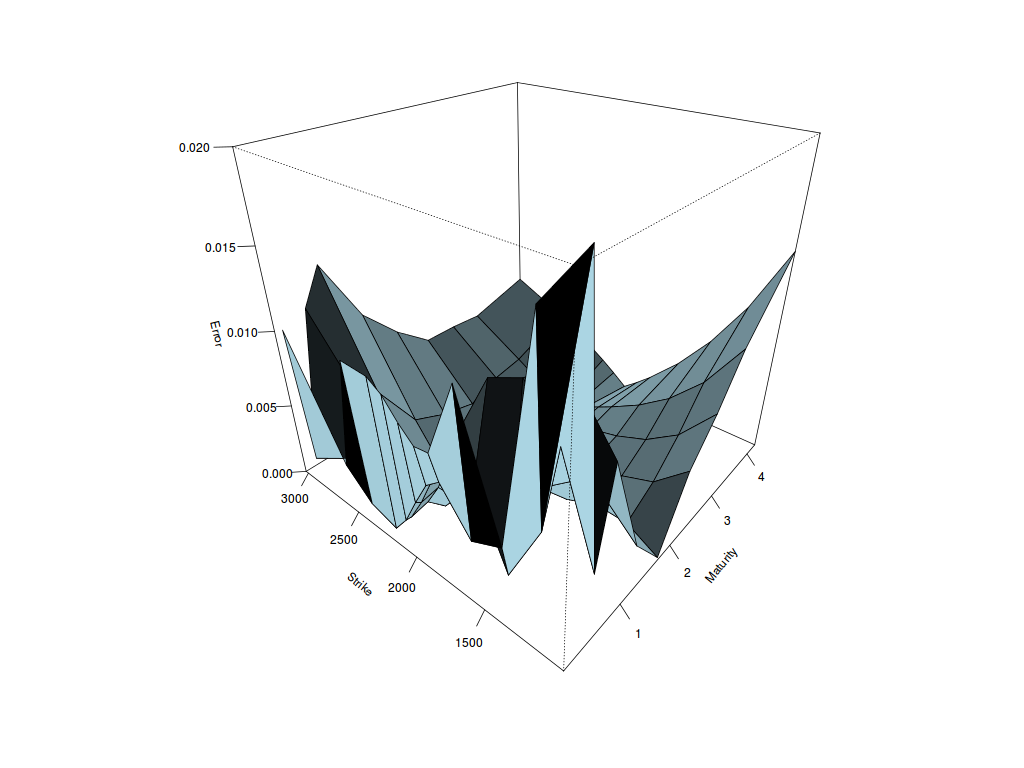
I did some experiments fitting Heston, Schobel-Zhu, Bates and Double-Heston to a real world equity index implied volatility surface. I used a global optimizer (differential evolution).
To my surprise, the Heston fit is quite good: the implied volatility error is less than 0.42% on average. Schobel-Zhu fit is also good (0.47% RMSE), but a bit worse than Heston. Bates improves quite a bit on Heston although it has 3 more parameters, we can see the fit is better for short maturities (0.33% RMSE). Double-Heston has the best fit overall but it is not that much better than simple Heston while it has twice the number of parameters, that is 10 (0.24 RMSE). Going beyond, for example Triple-Heston, does not improve anything, and the optimization becomes very challenging. With Double-Heston, I already noticed that kappa is very low (and theta high) for one of the processes, and kappa is very high (and theta low) for the other process: so much that I had to add a penalty to enforce constraints in my local optimizer. The best fit is at the boundary for kappa and theta. So double Heston already feels over-parameterized.
Heston volatility error
Schobel-Zhu volatility error
Bates volatility error
Double Heston volatility error
Another advantage of Heston is that one can find tricks to find a good initial guess for a local optimizer.
Update October 7: My initial fit relied only on differential evolution and was not the most stable as a result. Adding Levenberg-Marquardt at the end stabilizes the fit, and improves the fit a lot, especially for Bates and Double Heston. I updated the graphs and conclusions accordingly. Bates fit is not so bad at all.
I recently stumbled upon an error in the various papers related to the Heston Cos method regarding the second cumulant. It is used to define the boundaries of the Cos method. Letting phi be Heston characteristic function, the cumulant generating function is:
$$g(u) = \log(\phi(-iu))$$
And the second cumulant is defined a:
$$c_2 = g’’(0)$$
Compared to a numerical implementation, the c_2 from the paper is really off in many use cases.
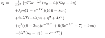
This is where Maxima comes useful, even if I had to simplify the results by hand. It leads to the following analytical formula:
$$c_2 = \frac{v_0}{4\kappa^3}{ 4 \kappa^2 \left(1+(\rho\sigma t -1)e^{-\kappa t}\right) + \kappa \left(4\rho\sigma(e^{-\kappa t}-1)-2\sigma^2 t e^{-\kappa t}\right)+\sigma^2(1-e^{-2\kappa t}) }\\+ \frac{\theta}{8\kappa^3} { 8 \kappa^3 t - 8 \kappa^2 \left(1+ \rho\sigma t + (\rho\sigma t-1)e^{-\kappa t}\right) + 2\kappa \left( (1+2e^{-\kappa t})\sigma^2 t+8(1-e^{-\kappa t})\rho\sigma \right) \\+ \sigma^2(e^{-2\kappa t} + 4e^{-\kappa t}-5) }$$
In contrast, the paper formula was:
I saw this while trying to calibrate Heston on a bumped surface: the results were very different with the Cos method than with the other methods. The short maturities were mispriced, except if one pushed the truncation level L to 24 (instead of the usual 12), and as a result one would also need to significantly raise the number of points used in the Cos method. With the corrected formula, it works well with L=12.
Here is an example of failure on a call option of strike, spot 1.0 and maturity 1.0 and not-so-realistic Heston parameters $$\kappa=0.1, \theta=1.12, \sigma=1.0, v_0=0.2, \rho=-0377836$$ using 200 points:
A few years ago, I found an interesting open source symbolic calculus software called Xcas. It can however be quickly limited, for example, it does not seem to work well to compute Taylor expansions with several embedded functions. Google pointed me to another popular open source package, Maxima. It looks a bit rudimentary (command like interface), but formulas can actually be very easily exported to latex with the tex command. Here is a simple example:
$$-{{\left(e^{t,\lambda}-1\right),\eta^2,x}\over{2,e^{t,\lambda},\lambda}}+{{\left(\left(4,e^{t,\lambda},t,\eta^3,\rho+\left(4,\left(e^{t,\lambda}\right)^2-4,e^{t,\lambda}\right),\eta^2\right),\lambda^2+\left(\left(-4,\left(e^{t,\lambda}\right)^2+4,e^{t,\lambda}\right),\eta^3,\rho-2,e^{t,\lambda},t,\eta^4\right),\lambda+\left(\left(e^{t,\lambda}\right)^2-1\right),\eta^4\right),x^2}\over{8,\left(e^{t,\lambda}\right)^2,\lambda^3}}+{{\left(\left(8,\left(e^{t,\lambda}\right)^2,t^2,\eta^4,\rho^2-16,\left(e^{t,\lambda}\right)^2,t,\eta^3,\rho\right),\lambda^4+\left(16,\left(e^{t,\lambda}\right)^2,t,\eta^4,\rho^2+\left(-8,\left(e^{t,\lambda}\right)^2,t^2,\eta^5+\left(16,\left(e^{t,\lambda}\right)^3-16,\left(e^{t,\lambda}\right)^2\right),\eta^3\right),\rho+16,\left(e^{t,\lambda}\right)^2,t,\eta^4\right),\lambda^3+\left(\left(-16,\left(e^{t,\lambda}\right)^3+16,\left(e^{t,\lambda}\right)^2\right),\eta^4,\rho^2+\left(-16,\left(e^{t,\lambda}\right)^2-8,e^{t,\lambda}\right),t,\eta^5,\rho+2,\left(e^{t,\lambda}\right)^2,t^2,\eta^6+\left(-8,\left(e^{t,\lambda}\right)^3+8,e^{t,\lambda}\right),\eta^4\right),\lambda^2+\left(\left(12,\left(e^{t,\lambda}\right)^3-12,e^{t,\lambda}\right),\eta^5,\rho+\left(2,\left(e^{t,\lambda}\right)^2+4,e^{t,\lambda}\right),t,\eta^6\right),\lambda+\left(-2,\left(e^{t,\lambda}\right)^3-\left(e^{t,\lambda}\right)^2+2,e^{t,\lambda}+1\right),\eta^6\right),x^3}\over{32,\left(e^{t,\lambda}\right)^3,\lambda^5}}+\cdots $$
Regarding Taylor expansion, there seems to be quite a few options possible, but I found that the default expansion was already relatively easy to read. XCas produced less readable expansions, or just failed.
I tried today the Scala courses on coursera by the Scala creator, Martin Odersky. I was quite impressed by the quality: I somehow believed Scala to be only a better Java, now I think otherwise. Throughout the course, even though it all sounds very basic, you understand the key concepts of Scala and why functional programming + OO concepts are a natural idea. What’s nice about Scala is that it avoids the functional vs OO or even the functional vs procedural debate by allowing both, because both can be important, at different scales. Small details can be (and probably should be) procedural for efficiency, because a processor is a processor, but higher level should probably be more functional (immutable) to be clearer, easier to evolve and more easily parallelized.
I recently saw a very good example at work recently of how mutability could be very problematic, with no gain in this case because it was high level (and likely just the result of being too used to OO concepts).
I believe it will make my code more functional programming oriented in the future, especially at the high level.
My Scala habits have made me create a stupid bug related to Java enums. In Scala, the concept of case classes is very neat and recently, I just confused enum in Java with what I sometimes do in Scala case classes.
I wrote an enum with a setter like:
public static enum BlackVariateType { V0, ZERO_DERIVATIVE;
private double volSquare; public double getBlackVolatilitySquare() { return volSquare; }
public void setBlackVolatilitySquare(double volSquare) { this.volSquare = volSquare; } }
Here, calling setBlackVolatilitySquare will override any previous value, and thus, if several parts are calling it with different values, it will be a mess as there is only a single instance.
I am not sure if there is actually one good use case to have a setter on an enum. This sounds like a very dangerous practice in general. Member variables allowed should be only final.
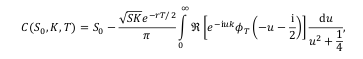
A coworker pointed to me that Andersen and Piterbarg book “Interest Rate Modeling” had a chapter on Fourier integration applied to Heston. The authors rely on the Lewis formula to price vanilla call options under Heston.
Lewis formula
More importantly, they strongly advise the use of a Black-Scholes control variate. I had read about that idea before, and actually tried it in the Cos method, but it did not improve anything for the Cos method. So I was a bit sceptical. I decided to add the control variate to my Attari code. The results were very encouraging. So I pursued on implementing the Lewis formula and their basic integration scheme (no change of variable).
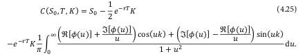
Attari formula
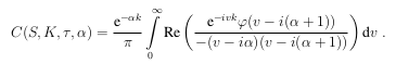
Carr-Madan formula (used by Lord-Kahl)
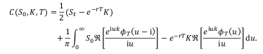
Heston formula
Cos formula
My impression is that the Lewis formula is not so different from the Attari formula in practice: both have a quadratic denominator, and are of similar complexity. The Lewis formula makes the Black-Scholes control variate real (the imaginary part of the characteristic function is null). The Cos formula looks quite different, but it actually is not that much different as the Vk are quadratic in the denominator as well. I still have this idea of showing how close it is to Attari in spirit.
My initial implementation of Attari relied on the log transform described by Kahl-Jaeckel to move from an infinite integration domain to a finite domain. As a result adaptive quadratures (for example based on Simpson) provide better performance/accuracy ratio than a very basic trapezoidal rule as used by Andersen and Piterbarg. If I remove the log transform and truncate the integration according by Andersen and Piterbarg criteria, pricing is faster by a factor of x2 to x3.
This is one of the slightly surprising aspect of Andersen-Piterbarg method: using a very basic integration like the Trapezoidal rule is enough. A more sophisticated integration, be it a Simpson 3/8 rule or some fancy adaptive Newton-Cotes rule does not lead to any better accuracy. The Simpson 3/8 rule won’t increase accuracy at all (although it does not cost more to compute) while the adaptive quadratures will often lead to a higher number of function evaluations or a lower overall accuracy.
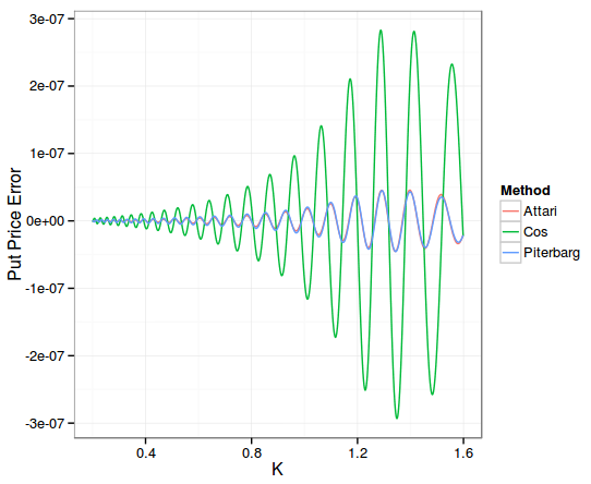
Here is the accuracy on put options with a maturity of 2 years:
I had to push to 512 points for the Cos method and L=24 (truncation) in order to have a similar accuracy as Attari and Andersen-Piterbarg with 200 points and a control variate. For 1000 options here are the computation times (the difference is smaller for 10 options, around 30%):
Method
Time
Attari
0.023s
Andersen-Piterbarg
0.024s
Cos
0.05s
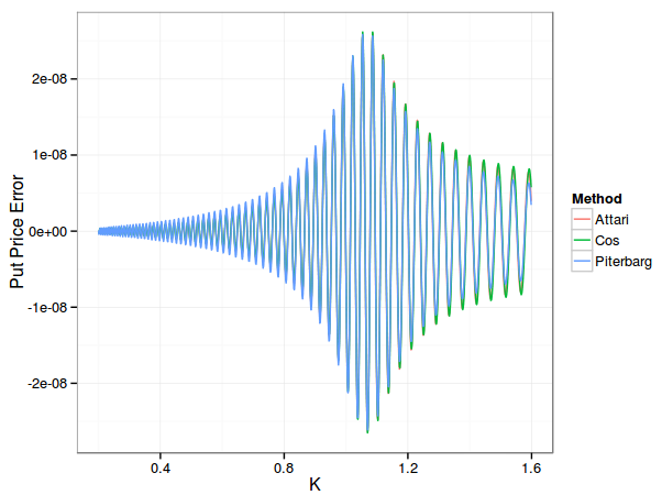
Here is the accuracy on put options with a maturity of 2 days:
All methods used 200 points. The error is nearly the same for all. And the Cos method takes now only 0.02s. The results are similar with a maturity of 2 weeks.
Conclusion
The Cos method performs less well on longer maturities. Attari or Lewis formula with control variate and caching of the characteristic function are particularly attractive, especially with the simple Andersen-Piterbarg integration.
I recently wrote about the Cos method. While rereading the various papers on Heston semi-analytical pricing, especially the nice summary by Schmelzle, it struck me how close were the Attari/Bates methods and the Cos method derivations. I then started wondering if Attari was really much worse than the Cos method or not.
I noticed that Attari method accuracy is directly linked to the underlying Gaussian quadrature method accuracy. I found that the doubly adaptive Newton-Cotes quadrature by Espelid (coteda) was the most accurate/fastest on this problem (compared to Gauss-Laguerre/Legendre/Extrapolated Simpson/Lobatto). If the accuracy of the integration is 1e-6, Attari maximum accuracy will also be 1E-6, this means that very out of the money options will be completely mispriced (might even be negative). In a sense it is similar to what I observed on the Cos method.
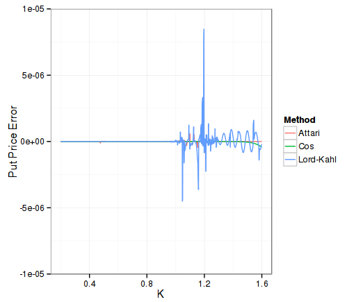
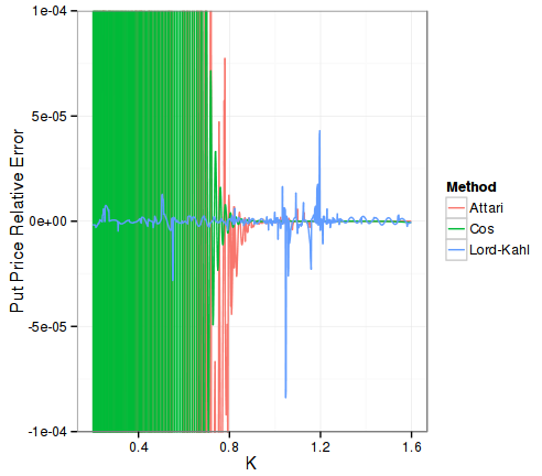
“Lord-Kahl” uses 1e-4 integration accuracy, “Attari” uses 1E-6, and “Cos” uses 128 points. The reference is computed using Lord-Kahl with Newton-Cotes and 1E-10 integration accuracy.
Well here are the results in terms of accuracy:
As expected, Lord-Kahl absolute accuracy is only 1E-5 (a bit better than 1E-4 integration accuracy), while Attari is a bit better than 1E-6, and Cos is nearly 1E-7 (higher inaccuracy in the high strikes, probably because of the truncation inherent in the Cos method).
The relative error tells a different story, Lord-Kahl is 1E-4 accurate here, over the full range of strikes. It is the only method to be accurate for very out of the money options: the optimal alpha allows to go beyond machine epsilon without problems. The Cos method can only go to absolute accuracy of around 5E-10 and will oscillate around, while the reference prices can be as low as 1E-25. Similarly Attari method will oscillate around 5E-8.
What’s interesting is how much time it takes to price 1000 options of various strikes and same maturity. In Attari, the charateristic function is cached.
Method
Time
Cos
0.012s
Lord-Kahl
0.099s
Attari
0.086s
Reference
0.682s
The Cos method is around 7x faster than Attari, for a higher accuracy. Lord-Kahl is almost 8x slower than Cos, which is still quite impressive given that here, the characteristic function is not cached, plus it can price very OTM options while following a more useful relative accuracy measure. When pricing 10 options only, Lord-Kahl becomes faster than Attari, but Cos is still faster by a factor of 3 to 5.
It’s also quite impressive that on my small laptop I can price nearly 100K options per second with Heston.