In reality, the problem is much simpler in the Bachelier/Normal model. A very basic analysis of Bachelier formula shows that the problem can be reduced to a single variable, as Choi et al explain in their paper. So the problem is not really one of solving, but one of approximating (the inverse of) a function.
The first step to build that function is to actually have a highly accurate slow solver as reference. This is quite easy, I just started with Choi formula and used Halley's method to refine. In reality, Halley's method is already a bit overkill on this problem: it works impressively well, 1 iteration is enough to have an insane level of accuracy, only noticeable when one works in high precision arithmetic (for example 50 digits). For double precision, Newton's method would actually be enough - I initially thought that my Halley's implementation did not work as it produced the exact same output as Newton in double precision. Li proposes the use of the SOR method, which for this exercise, behaves very much like Newton's method.
I then followed the logic from Choi et al, but working directly with in-the-money call options instead of straddles. Straddles sound neat at first (hides that we work in-the-money), but it's actually useless for the algorithm. Choi et al. ignore half of the straddle range when they use their eta transform in the paper. One other change is the mapping itself, I found a better mapping for the call options (but not that far of Choi initial idea). Finally, because I am lazy, I did not go to the pain of finding a good rational fraction approximation along with the square root problem they describe, I just tried a Chebyshev polynomial.
Unfortunately, a single Chebyshev polynomial does not work well: even with a very large (1000) degree it's not very precise, so much that I thought that my transform was garbage. I had noticed by mistake, that on another part (negative) of the interval, the Chebyshev polynomial worked actually very well to approximate something related to the volatility of another option. Suddendly came to me the idea of, like Johnson does in his Faddeeva package, using N Chebyshev polynomials on N small intervals. This is like the big heavy hammer for which everything looks like nails, but it's actually very fast to evaluate as the degree of each polynomial can then be low (7), plus a table lookup (could be coded as switch statements if one really cares about such details). The slowest part is actually the call to the log function.
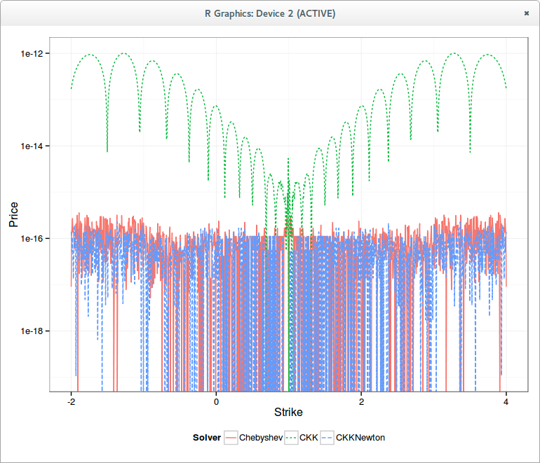
The final bit is the use of a Taylor approximation for my -u/log(1-u) transform as it is not all that accurate in double precision when u is near 0. And that produces the following graph
It is interesting to note that "solving" the b.p. vol is 10x faster than solving the Black vol.
The calibration of a stochastic volatility model or a volatility surface parameterization (like SVI) involves minimizing the model options volatilities against market options volatilities. Often, the model computes an option price, not an implied volatility. It is therefore useful to have a fast way to invert that option price to get back the implied volatility that corresponds to it. Furthermore during the calibration procedure, the model option price can vary widely: it is convenient to have a robust implied volatility solver.
Another more basic use of implied volatility solvers, is for the computation of Black-Scholes greeks for a given market option price.
A few years ago, P. Jaeckel produced a much better algorithm than a simple Newton or Brent solver, in his paper By Implication. There is also a much simpler algorithm from Li, based on SOR and a good initial guess for SOR, which I found to be actually quite robust and fast. Now P. Jaeckel has a newer algorithm, faster and more accurate, close to double accuracy.
I have tested those on 1 million options of random volatility (between 0.001 and 3), random strikes (N deviations with a cap at 1M) for a few expiries.In terms of performance, the results are independent of expiries, but in terms of accuracy, the new Jaeckel algorithm is particularly more accurate for the long-term options (5y and 15y).
Algorithm
Expiry
Vol RMSE
Price RMSE
Time
Jaeckel2014
5y
3.8E-16
2.1E-16
1.8s
Jaeckel2006
5y
1.3E-10
1.1E-10
3.0s
Jaeckel2014
15y
2.0E-12
2.4E-16
1.8s
Jaeckel2006
15y
1.5E-7
8.0E-11
2.7s
The maximum error from Jaeckel2006 is around 1e-8, while the one from Jaeckel2014 is 2e-15 (for very large unrealistic strike)
As a comparison, the simpler Li SOR-TS algorithm follows the given price accuracy independently of the expiry; I have tested with 1E-12. The error in implied volatility will be slightly higher: different close vols can give the same price due to the maximum achievable accuracy of the Black-Scholes formula with double numbers, even with a good cumulative normal distribution implementation. Its performance is however dependent on the number of deviations considered: closer to ATM means faster for Li algorithm.<
Algorithm
Expiry
Deviation
Vol RMSE
Price RMSE
Time
Jaeckel2014
1y
5
4.2E-16
2.0E-17
1.8s
LiSORTS
1y
5
8.5E-9
1.9E-13
2.1s
Jaeckel2014
1y
3
3.1E-16
5.9E-17
1.7s
LiSORTS
1y
3
4.3E-12
1.6E-13
1.3s
Actually, I have cheated in my Li SOR-TS implementation: I have reused the idea from P. Jaeckel to compute the Black-Scholes price with erfc_x (unscaled erfc) instead of erfc. This simple change divides the number of exp calls by 2. Without this trick, for 5 deviations, SOR-TS took 3.6s (almost twice the time).
I would not be surprised if this was the main performance improvement between the two Jaeckels.
Tension splines can produce in some cases arbitrage free C2 interpolation of options, but unfortunately this is not guaranteed. It turns out that, on some not so nice looking data, where the discrete probability density is not monotone but only positive, all previously considered interpolation fail (spline in volatility or variance, tension spline in log prices, harmonic spline on prices).
K
vol
put
b-slope
b-convexity
300.0
0.682
0.090
0.00e+00
0.00e+00
310.0
0.654
0.136
4.60e-03
0.00e+00
320.0
0.621
0.192
5.60e-03
1.00e-03
330.0
0.594
0.288
9.60e-03
4.00e-03
340.0
0.560
0.404
1.16e-02
2.00e-03
350.0
0.520
0.530
1.26e-02
1.00e-03
360.0
0.484
0.736
2.06e-02
8.00e-03
370.0
0.467
1.232
4.96e-02
2.90e-02
380.0
0.442
1.898
6.66e-02
1.70e-02
390.0
0.427
3.104
1.21e-01
5.40e-02
400.0
0.412
4.930
1.83e-01
6.20e-02
Possibly the simplest arbitrage free interpolation is to postulate the density as piecewise constant, ideally centered around each strike (if not centered, there is no guarantee that it will be positive). If a spline is used for interpolation, this means a quadratic spline. Unfortunately, because it is not C2, it then still fails to be arbitrage free.
It is also possible to price by integrating the payoff over the density. There is then one degree of freedom, the Fmin (minimum forward allowed before absorption) that can be adjusted so as to make the density always positive. This produces our only arbitrage free interpolation of the above input put option prices.
The implied volatility looks reasonable on this strange input: very much like a spline on volatilities. In contrast, the parabolic interpolator produces an oddly looking implied volatility shape, even though the density is in a way similar: piecewise constant. This is likely because I forced the second derivatives to match the discrete curvature, it is then not C1 in prices.
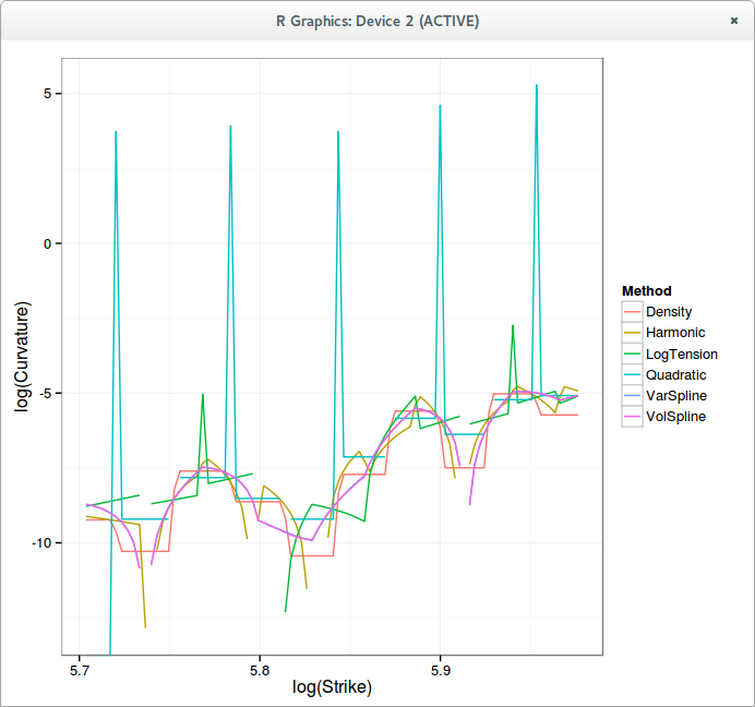
Unfortunately, the piecewise constant density interpolant can also produce some strange implied volatility shapes, for example on P. Jaeckel example data:
We find back the wiggles for large strikes. The lower end is particularly funny (which could be due to the fact that I don’t have the data for low strikes). This is the corresponding density:
It appears then not so easy to produce a simple generally good looking interpolation.
In a previous post, I have explored the arbitrage free wiggles in the volatility surface that P. Jaeckel found in his paper. I showed that interpolating in log prices instead of prices was enough to remove the wiggles, but then, it appears that the interpolation is not guaranteed to be arbitrage free, even though it often is. On another example from P. Jaeckel paper, that I reproduced inaccurately but well enough, it is not.
Using a Harmonic spline instead of a regular cubic spline seems to be enough to make the interpolation arbitrage free in practice (although not in theory as log-prices are not convex), but it is only C1.
One can use a tension spline instead. There is an algorithm from Pruess that updates the tension parameters so as to make the interpolation monotone and convex. It can be tweaked to ensure that the interpolation follows:
$$f’^2 + f’’ \geq 0$$
This condition makes the interpolation on the log prices arbitrage free. As a first draft experiment, I just ensured numerically that the condition was valid, the resulting algorithm was fast enough and worked reasonably well.
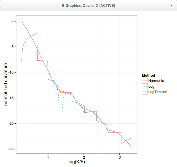
Here is how the normalized density looks like with a simple harmonic spline on the call prices, a cubic spline in the logarithm of call prices, and an optimized tension spline in the logarithm of call prices.
logarithm of the curvature
The blank spot for the Log curve (spline) corresponds to negative curvature, that is, arbitrage. Notice how the tension spline is fully continuous, with no real spikes.
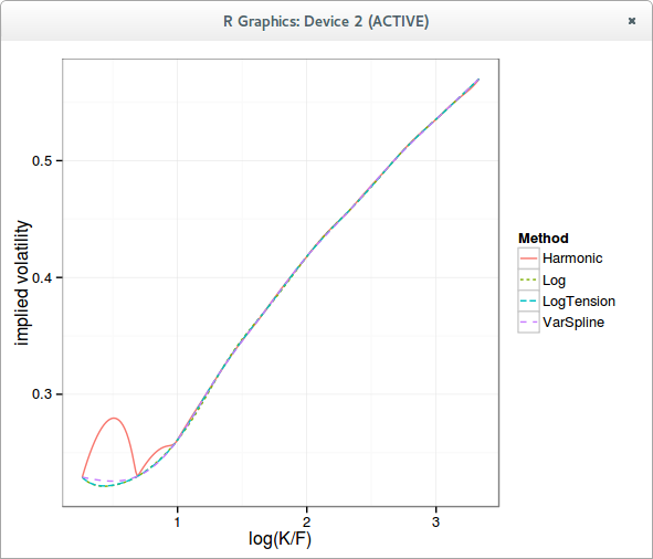
The implied volatility curve is very close to a more classic cubic spline interpolation on the implied variance.
Of course, the same kind of algorithm can be applied directly to the variance with a slightly different numerical test to ensure it is arbitrage-free, it might however be easier to find a more robust and more clever algorithm in the log prices.
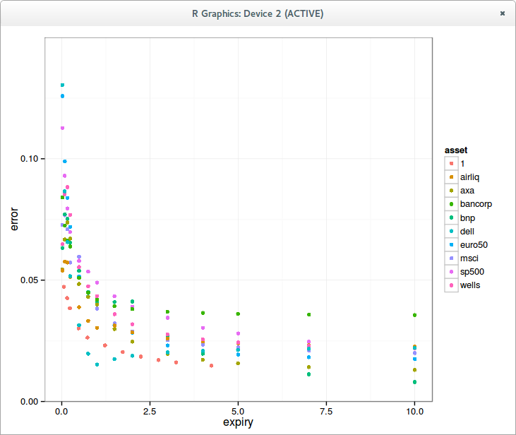
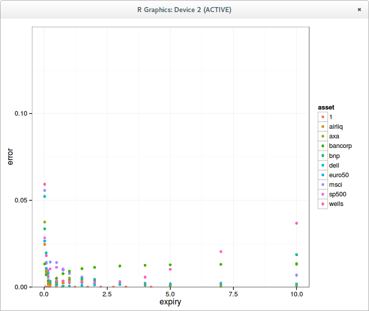
I always wondered if Bachelier was really worse than Black-Scholes in practice. As an experiment I fit various implied volatility surfaces with Bachelier and Black-Scholes and look at the average error in implied volatility by slice.
In theory Bachelier is appealing because slightly simpler: log returns are a bit more challenging to think about than returns. And it also takes indirectly into account the fact that OTM calls are less likely than OTM puts because of default risk, if you assume absorbing probability at strike 0.
Bachelier
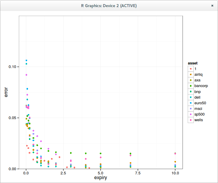
Black-Scholes
The error is in general smaller for Black-Scholes for short expiries, and higher for long expiries when compared to Bachelier. Interestingly, in theory, the difference of the models is more pronounced for longer expiries. One would have imagined that for very short expiries Bachelier would be equivalent to Black, it is not the case in term of fitting the smile.
Displaced diffusion (mixing both Bachelier and Black linearly) allows to gain x2 accuracy.
Displaced Diffusion
What about SABR? Let's look at lognormal SABR, usually used for equities.
Lognormal SABR (beta=1)
The fit is much better for long expiries, but not so great for a few outliers for long maturities, it can be actually worse than the simple displaced diffusion. A normal SABR might fix that.
Normal SABR (beta=0) using Hagan lognormal formula
If one relies on the standard lognormal formula, the beta=0 SABR behaves very badly.
Normal SABR using Hagan normal formula
This is fixed using the normal (bpvol) Hagan formula directly. The fit is then better overall for long maturities as expected from Black-Scholes vs Bachelier behavior.
If one look in log scale, the conclusion is not so obvious: beta=1 produces a better fit for a majority even for long expiries, but worse for a few (30% in my case) outliers.
What's clear however, is that one should never use the Black implied volatility Hagan formula with beta=0. This leaves a question on displaced SABR. Is displaced SABR is better suited than SABR with varying beta?
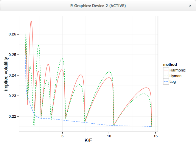
Peter Jaeckel, in a recent paper (pdf), shows that something that sounds like a reasonable arbitrage free interpolation can produce wiggles in the implied volatility slice.
The interpolation in question is using some convexity preserving spline on call and put option prices directly and in strike, assuming those input prices are arbitrage free. This is very similar to Kahale interpolation (pdf).
It seemed too crazy for me so I had to try out his example. And using a harmonic spline, it does produce arbitrage free wiggles.
Wiggles in the implied volatility
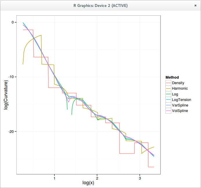
If we look at the probability density (the curvature), the Harmonic spline maintains a positive density, nearly piecewise flat in log scale, while Hyman, because it preserves only monotonicity, has some negative density which are cut out from the graph.
Probability Density
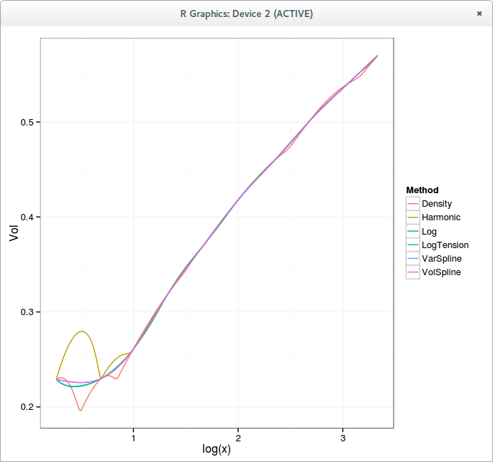
In reality, if we look at the interpolation of prices in log scale, one can see that splines won't behave as expected at first on small numbers: they will give a much higher weight to the high values, producing something like a piecewise linear interpolation.
In reality, what one really wants for such data is to just interpolate the log prices with a spline, not the prices. This is the curve named "Log" in the graphs, where a simple cubic spline is used on the log prices, and fed to exp after interpolation.
Now it sounds like a reasonable arbitrage free interpolation would be to interpolate the discrete density log linearly, in a similar spirit as Hagan-West yield curve interpolation (pdf).
In general, if you interpolate very small numbers with a spline, you probably are doing something wrong.
In an earlier post, I have been quickly exploring adjoint differentiation in the context of analytical Black-Scholes. Today, I tried to mix it in a simple Black-Scholes Monte-Carlo as described in L. Capriotti paper, and measured the performance to compute delta compared to a numerical single sided finite difference delta.
I was a bit surprised that even on a single underlying, without any real optimization, adjoint delta was faster by a factor of nearly 40%. I suspect this is mostly due to exp evaluations being /2.
On a basket of 4 assets, the adjoint method was 3.25x faster.
It’s quick to have such results on basic payoffs: it took me a few hours and worked on the first run, even though my Monte-Carlo is slightly different from the Capriotti paper. It is much more challenging to have it working across a wide variety of payoffs, and to automatize some of it.
Several papers show that the limit for large strikes of Heston is SVI.
Interestingly, I stumbled onto a surface where the Hagan SABR fit was perfect as well as the SVI fit, while the Heston fit was not.
Originally, I knew that, on this data, the SVI fit was perfect. Until today, I just never tried to fit a lognormal SABR on the same data. I did a small test with random values of the SABR parameters alpha, rho, nu, and found out that in deed, the SVI fit is always perfect on SABR.
Is this just because the Taylor expansion of SVI will match the Taylor expansion of SABR up to the fourth order? It seems that the wings are also not too far off in general so there could be more to it.
Gatheral actually devised an SVI formula that uses SABR like variables in a talk here.
Of course, the reverse is not true. SVI has more parameters and provides in general a better fit than SABR.
With a small time expansion, it is easy to derive a reasonable initial guess, without resorting to some global minimizer.
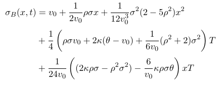
Like Forde did for Heston, one can find the 5 Schobel-Zhu parameters through 5 points at coordinates (0,0), (x0,t1), (-x0,t1), (x0,t2), (-x0,t2), where x0 is a chosen the log-moneyness, for example, 0.1 and t1, t2 relatively short expiries (for example, 0.1, 0.25).
We can truncate the small time expansion so that the polynomial in (x,t) is fully captured by those 5 points. In practice, I have noticed that using a more refined expansion with more terms resulted not only in more complex formulas to lookup the original stochastic volatility parameters, but also in an increased error, because of the redundancy of parameters in the polynomial expansion. My previous Schobel-Zhu expansion becomes just:
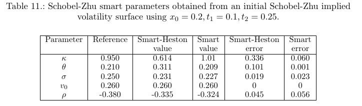
In practice, I have found that the procedure works rather well.
On some more extreme surfaces, where theta=0, the error in kappa and theta is higher. Interestingly, I received a few real world surfaces like this, where theta=0, which I found a bit puzzling. I wondered if it was because those surfaces were preprocessed with SABR, that has no mean reversion, but I could not fit those exactly with SABR.
Small time expansions for Heston can be useful during the calibration of the implied volatility surface, in order to find an initial guess for a local minimizer (for example, Levenberg-Marquardt). Even if they are not so accurate, they capture the dynamic of the model parameters, and that is often enough.
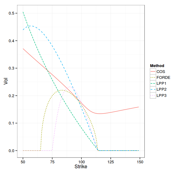
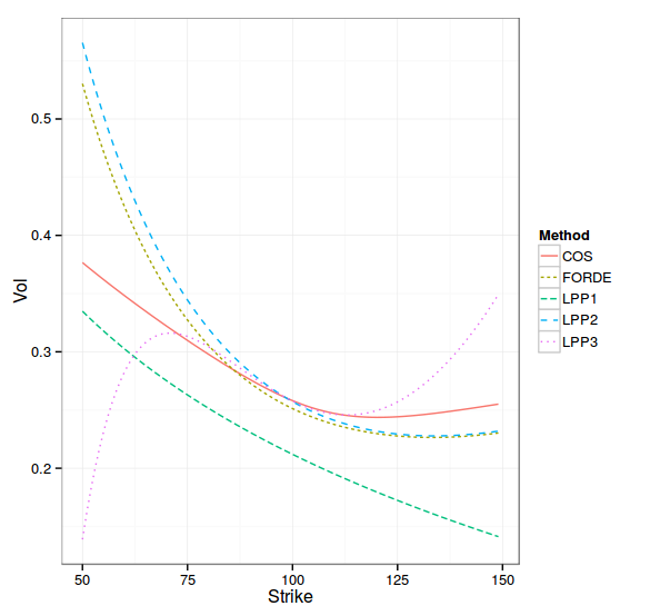
I noticed, however, that on some surfaces, the Lorig expansion was quickly very inaccurate (LPP1 for order-1, LPP2 for order-2, LPP3 for order-3). Those surfaces seem to be the ones were the Feller condition is largely violated. In practice, in my set of volatility surfaces for 10 different equities/indices, the best fit is always produced by Heston parameters where the Feller condition is violated.
T=0.5, Feller condition largely violated
T=0.5, Feller condition slightly violated
Out of curiosity, I calibrated my surfaces feeding the order-1 approximation to the differential evolution, in order to find my initial guess, and it worked for all surfaces.
The order-3 formula, even though it is more precise at the money, was actually more problematic for calibration: it failed to find a good enough initial guess in some cases, maybe because the reference data should be truncated, to possibly keep the few shortest expiries, and close to ATM strikes.